Karamea flood tutorial
From Gerris
This page is a step-by-step description of how to setup, run and visualise a flood simulation using the GfsRiver solver of Gerris.
Contents |
Prerequisites
I will assume that you have access to a machine where both Gerris and GfsView are installed. All the commands described in this tutorial need to be run on this system.
We will start by creating a directory
% mkdir karamea
% cd karamea
We will simulate the lower reaches of the Karamea river, including part of the sea on the western boundary. Three input files are thus required:
- A Digital Terrain Model of the area:
topo.asc - A flow-rate file defining the evolution in time of the river flow at the eastern boundary:
flow.asc - A tide file defining the sea level at the western boundary:
tide.asc
These files need to be copied to our karamea directory.
All files should be in Unix ASCII format. If they have been created on a Windows system, they should be converted using:
% dos2unix topo.asc flow.asc tide.asc
We will assume that the DTM file uses the ESRI grid ASCII format. The file should look like:
% more topo.asc
ncols         1867
nrows         1490
xllcorner     1523880
yllcorner     5430180
cellsize      3
NODATA_value  -9999
19 19 1...
The flow.asc and tide.asc files are lists of two values separated by a space or tab. The first is the time in hours, the second the value of either the flow rate (in cumecs) or the sea level (in metres relative to zero). The files should look like:
% more flow.asc
0.00	151.5
1.00	176.63
2.00	463.7
3.00	1013.93
4.00	1306.4
5.00	1709.67
6.00	2320.75
...
Setting up the simulation domain
We first need to write a parameter file for Gerris. Use your favourite text editor and cut and paste the following
1 0 GfsRiver GfsBox GfsGEdge {} {
}
GfsBox {}
then save the file as karamea.gfs. This is the smallest valid Gerris parameter file possible. It just says that we want to use the GfsRiver model and that the simulation domain is a single "GfsBox", by default a square centered on (0,0) and of size unity i.e. the coordinates of the simulation domain are within [-0.5:0.5] x [-0.5:0.5]. We can then run this simulation using
% gerris2D karamea.gfs
Of course this doesn't do much yet... We first need to make the domain larger. Our topo.asc file defines a domain width of 1867 x 3 = 5601 metres, so we will set the box size to 5600 metres by adding
1 0 GfsRiver GfsBox GfsGEdge {} {
    PhysicalParams { L = 5600 g = 9.81 }
}
GfsBox {}
Note that we have also defined the acceleration of gravity (in m/s^2). Gerris doesn't impose any units by default; it's up to the user to define quantities in a consistent unit system. By defining g to 9.81 we are now forced to specify any other length using metres and any other time using seconds. For example, the following would have also been valid
PhysicalParams { L = 5.6 g = 0.00981 }
but all lengths should now be specified in kilometres (times still in seconds). A slighty more complex example would be
PhysicalParams { L = 5.6 g = 127137.6 }
where all lengths now use kilometres and times use hours (g is now in km/hour^2).
For this tutorial, we have to stay in metres and seconds to be consistent with our input files above. We then have a domain with coordinates within [-2800:2800] x [-2800:2800]. It would be nice to recenter everything in [0:5600] x [0:5600] so that our domain matches the terrain model in topo.asc. This can be done using
1 0 GfsRiver GfsBox GfsGEdge { x = 0.5 y = 0.5 } {
    PhysicalParams { L = 5600 g = 9.81 }
}
GfsBox {}
which shifts the position of the center of the square to (0.5,0.5) (before resizing the domain, so that the bottom-left corner of the domain is now at (0,0)). To work in absolute coordinates, we need to further shift this origin to the origin of the terrain model (the xll,yll parameters of topo.asc). This can be done using
1 0 GfsRiver GfsBox GfsGEdge { x = 0.5 y = 0.5 } {
    PhysicalParams { L = 5600 g = 9.81 }
    MapTransform { tx = 1523880 ty = 5430180 }
}
GfsBox {}
Creating the topography
To be able to generate the topography we first need to convert topo.asc to the Gerris terrain database format. This database does not depend on the detail of the Gerris model. For example the same terrain database can be used for models running at different resolutions, smaller or larger domains or even different models (e.g. ocean models, 3D atmospheric models etc...). Several databases (corresponding for example to different datasets e.g. acoustic sounding bathymetry, lidar data, satellite altimetry etc...) can also be merged to create a single terrain. See the documentation for the Terrain module for more background info.
Gerris terrain databases are created using the xyz2kdt command. Like any other Gerris command (and many Unix commands), a simple explanation of the command can be obtained by typing
% xyz2kdt -h
Usage: xyz2kdt [OPTION] BASENAME

Converts the x, y and z coordinates on standard input to a
2D-tree-indexed database suitable for use with the
terrain module of Gerris.

  -p N  --pagesize=N  sets the pagesize in bytes (default is 4096)
  -v    --verbose     display progress bar
  -h    --help        display this help and exit

Report bugs to popinet@users.sf.net
xyz2kdt takes a list of space-separated triplets (x,y and z) as input. The first step is thus to convert topo.asc to such a list. Many tools can do this conversion (GIS systems for example). A simple and general way of doing such "text to text" conversions is to use the awk scripting language. Programming in awk is beyond the scope of this tutorial but the following should give you can idea of how this works. Open your text editor and cut and paste the following
BEGIN {
    n = 0;
}
{
    if ($1 == "ncols")
        ncols = $2;
    else if ($1 == "nrows")
        nrows = $2;
    else if ($1 == "xllcorner")
        x = xllcorner = $2;
    else if ($1 == "yllcorner")
        yllcorner = $2;
    else if ($1 == "cellsize") {
        cellsize = $2;
        y = yllcorner + cellsize*(nrows - 1);
    }
    else if ($1 == "NODATA_value")
        NODATA_value = $2;
    else
	for (i = 1; i <= NF; i++) {
	    if ($i != NODATA_value)
		printf ("%f %f %f\n", x,y,$i);
	    x += cellsize;
	    n++;
	    if (n >= ncols) {
		print "";
		y -= cellsize;
		x = xllcorner;
		n = 0;
	    }
	}
}
Save the file as asc2xyz.awk. If you have done some programming you can guess what this code does. It just retrieves the header information from the ESRI ASCII grid file and computes the corresponding x,y coordinates for each data value.
We can check whether this works using
% awk -f asc2xyz.awk < topo.asc | more
1523880.000000 5434647.000000 19.000000
1523883.000000 5434647.000000 19.000000
1523886.000000 5434647.000000 19.000000
1523889.000000 5434647.000000 19.000000
1523892.000000 5434647.000000 19.000000
...
which looks OK.
To create the Gerris terrain database we could do
% awk -f asc2xyz.awk < topo.asc > topo.xyz
% xyz2kdt -v topo < topo.xyz
however we don't need to waste disk space by generating the topo.xyz file and we can use Unix pipes instead and do everything at once
% awk -f asc2xyz.awk < topo.asc | xyz2kdt -v topo
At this stage it is a good idea to check the statistics returned by xyz2kdt. In particular any inconsistency in the minimum, average and maximum height values:
2781830 points Height min: -9.43687 average: 10.9881 max: 33.79
can reveal errors in the input data.
We now have several files (in addition to the original topo.asc file) which together define the terrain database
% ls -lh topo*
-rw-r--r-- 1 popinet popinet 129K 2010-09-08 11:48 topo.kdt
-rw-r--r-- 1 popinet popinet  64M 2010-09-08 11:48 topo.pts
-rw-r--r-- 1 popinet popinet 2.9M 2010-09-08 11:48 topo.sum
Testing the database
To test whether this worked we will start by reconstructing and displaying the terrain corresponding to our simulation. One way of doing this is to add the following lines to our Gerris parameter file
1 0 GfsRiver GfsBox GfsGEdge { x = 0.5 y = 0.5 } {
    PhysicalParams { L = 5600 g = 9.81 }
    MapTransform { tx = 1523880 ty = 5430180 }
    GModule terrain
    RefineTerrain 8 T { basename = topo } TRUE
}
GfsBox {}
The terrain database system is a module of Gerris which we need to include (hence the GModule line). The RefineTerrain line specifies how to refine the mesh and the name of the variables which will hold the terrain representation. We set a maximum of eight levels of refinement: level 0 is the "root" of the quadtree i.e. the entire square domain, level 1 is obtained by dividing level 0 into four square cells, etc... thus eight levels of refinement will give 2^8 = 256 x 256 square cells.
If you haven't already you should follow the links to terrain and RefineTerrain above and have a read. Most keywords used in Gerris parameter files are documented in the syntax reference page.
We could now run this simulation but it would not do much because we have not told Gerris to output anything yet. To do this we add
1 0 GfsRiver GfsBox GfsGEdge { x = 0.5 y = 0.5 } {
    PhysicalParams { L = 5600 g = 9.81 }
    MapTransform { tx = 1523880 ty = 5430180 }
    GModule terrain
    RefineTerrain 8 T { basename = topo } TRUE
    OutputSimulation { start = end } stdout
}
GfsBox {}
So that the entire simulation is written on the standard output (stdout) at the end of the simulation (start = end). We can then do
% gerris2D karamea.gfs > end.gfs
Wait for a while and you will get a file looking like
% more end.gfs
# Gerris Flow Solver 2D version 1.3.2 (090819-232634)
1 0 GfsRiver GfsBox GfsGEdge { x = 0.5 y = 0.5 version = 90819 variables = P,U,V
,Zb,H,Px,Py,Ux,Uy,Vx,Vy,Zbx,Zby,T0,T1,T2,T3,Te,Tn,Tdmin,Tdmax binary = 1 } {
  # when editing this file it is recommended to comment out the following line
  GfsDeferredCompilation
  GModule terrain
  GfsTime { i = 3 t = 1.79769e+308 }
  ....
which is a Gerris parameter file which also contains the values of all variables listed after variables = . This file can be used to restart a simulation and can be visualised with GfsView:
% gfsview2D end.gfs
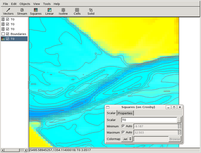
In the toolbar click on "Squares", select "Edit -> Properties" in the menu (or double-click on the icon in the left-hand pane), change "P" to "T0" in the dialog box (hit Enter when you have finished typing). You can then zoom by holding down the middle mouse button of (or using the scrollwheel), and drag by holding down the right mouse button. You should get something looking like this
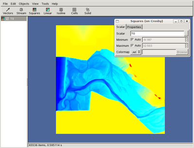
Also, holding down the Ctrl key while clicking on the left mouse button will display the (x,y) coordinates and the value of the selected field (e.g. T0) in the status bar.
Isolines can also be useful to check that the terrain has been correctly reconstructed. Playing with the "Isoline" object and its properties, you should be able to get something like this
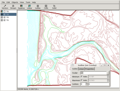
where the green line is the coast (T0 = 0), brown is above and blue is below sea level.
Can we save all the hard work spent setting up the visualisation within GfsView? Of course! just select "File -> Save" and type "isolines.gfv" in the "Path" dialog box and click on the "Save" button. Now select "Edit -> Clear", then "File -> Open", navigate and select "isolines.gfv" then click on "Ok" and you should be back where you started. The ".gfv" extension stands for GfsView and indicates that the file contains visualisation parameters for GfsView.
This file could also be used like this
% gfsview2D end.gfs isolines.gfv
Adaptive mesh generation
Using the "Cells" object in GfsView, you can see the mesh used to discretise the domain. As expected this is a regular Cartesian mesh with a resolution of 5600/256 ~ 22 metres. We could increase the resolution just by increasing the number of levels of refinement to, say, 10 which would give a resolution of 5600/2^10 ~ 5.5 metres. We can do better than this however and use an adaptive mesh where the resolution is increased only where necessary. To do this, just change the RefineTerrain line to
RefineTerrain 10 T { basename = topo } (Te > 0.1)
We have increased the maximum level of refinement to 10, but we have also changed the refinement condition from TRUE to (Te > 0.1). Te is the least-mean-square terrain reconstruction error. This means that the mesh will be refined (but no more than 10 levels) only when the terrain reconstruction error is larger than 0.1 metre. We can now test this using
% gerris2D karamea.gfs | gfsview2D -s isolines.gfv
Be patient while Gerris creates the terrain (it will take 10-20 seconds). Here we have used another Unix pipe trick where the solution generated by Gerris is directly fed into GfsView. The "-s" option tells GfsView to "survive" even when the unix pipe is "broken" (as happens when Gerris completes).
You can now use the "Cells" object in the toolbar of GfsView to visualise the variable-resolution mesh. Another useful way of doing this is to use the "Squares" object and replace "P" with "Level" which is the local level of refinement. This gives figures like this
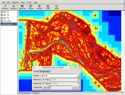
which are clearer for high-resolution meshes.
Note that the refinement condition is not limited to simple expressions. In fact, it can be anything from a constant (e.g. TRUE as in our initial test) to a complex C routine returning TRUE or FALSE. For example, imagine we want to generate a mesh with a terrain error of 5 cm in a radius of 400 metres around the center of the Karamea township but only 0.5 metre elsewhere. In our coordinate system the center of the Karamea township is roughly at (1525440,5433192). We could then use the following
RefineTerrain 10 T { basename = topo } {
  /* coordinates relative to the township center */
  x -= 1525440; y -= 5433192;
  if (x*x + y*y < 400*400)
    return (Te > 0.05);
  else
    return (Te > 0.5);
}
Rerunning with
% gerris2D karamea.gfs | gfsview2D -s isolines.gfv
will give something like this
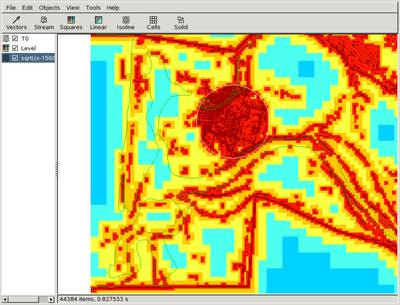
(how to draw the white circle around the township is left as an exercise for the reader...)
Setting inflow conditions
The inflow is defined by the flow.asc file which describes the variation in time of the river flow. However it is often a good idea to start with the simplest possible simulation and to add complexity bit by bit. In this spirit, we will start by imposing a constant inflow (no variation in time) of 2000 cumecs. This can be done using GfsDischargeElevation to compute the water level along a boundary which will ensure a given discharge. This water level can then be imposed as a boundary condition to obtain the discharge sought. This can be done using the following parameter file
1 0 GfsRiver GfsBox GfsGEdge { x = 0.5 y = 0.5 } {
    PhysicalParams { L = 5600 g = 9.81 }
    MapTransform { tx = 1523880 ty = 5430180 }
    GModule terrain
    RefineTerrain 8 T { basename = topo } (Te > 0.1)
    Init {} { Zb = T0 }

    DischargeElevation E 2000

    OutputTime { istep = 1 } stderr
    OutputSimulation { step = 10 } stdout
}
GfsBox {
    right = Boundary {
        BcDirichlet P MAX(E - Zb,0.)
    }
}
In addition to the terrain generation we already know, we added five lines:
-
Init...: the variable which defines the topography for a GfsRiver simulation is calledZb. We just set this variable to be equal toT0. We do that only once at the start of the simulation. -
DischargeElevation: defines a new variable (calledE) containing the water level we need to set on the boundary to obtained a discharge of 2000 cumecs. -
OutputTime...: the time is written to standard error at every timestep. -
OutputSimulation...: we have changed when outputs of the simulation are performed. They are now done every 10 seconds (of simulated time). -
BcDirichlet P MAX(E - Zb,0.): here we set the water level on the right-hand-side boundary toE. Because the water level is only a diagnostic variable, we do this indirectly by setting the water depthPtoE - Zb. TheMAXfunction just chops off any (non-physical) negative values.
If we now save this as karamea.gfs and do
% gerris2D karamea.gfs | gfsview2D isolines.gfv
we will get an output looking like
step:       0 t:      0.00000000 dt:  1.000000e+01 cpu:      0.00000000 real:      0.00000300
step:       1 t:     10.00000000 dt:  1.111111e+00 cpu:      0.17000000 real:      0.23817900
step:       2 t:     11.11111111 dt:  1.269841e+00 cpu:      0.34000000 real:      0.67936700
step:       3 t:     12.38095238 dt:  1.523810e+00 cpu:      0.46000000 real:      0.80351100
...
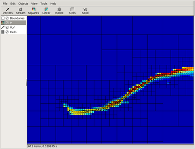
GfsView will receive new simulations every 10 seconds of simulated time. We can display the evolving solution by selecting "Squares", which will display "P" (the water depth) by default. Selecting "Vectors" will display the flux vectors. We need to pan and zoom to display the upstream boundary (the terrain is still "dry" downstream) and we get something like this

which looks alright although we may not have expected the river to fill as much of the riverbed close to the inflow. We will need to visualise this flow again later, so save the GfsView parameter file as flow.gfv.
We can have more control over how the specified discharge is distributed along the boundary. As explained in the documentation for DischargeElevation, we can specify an optional reference water level. For example, if we want to restrict the discharge to the main river channel, we can define the reference level to zero in the main channel and a large negative value elsewhere, so that the water level at the boundary will always be below the level of the topography outside of the main channel. The reference level is defined using a function of the spatial coordinates (x,y) along the boundary. We could work out what this function is using geographical coordinates, however for this particular example it is simpler to just visualise the terrain and construct this function interactively using GfsView. To do this we can use the end.gfs simulation we generated above and visualise it using GfsView:
% gfsview2D end.gfs isolines.gfv
We want to impose the inflow close to the right-hand-side boundary of the domain. Pan and zoom to display this part of the domain, then select "Objects -> Mesh -> Boundaries", click on "Squares", change "P" to "T0" and you should get something looking like this
which shows the right-hand-side boundary together with the upper reaches of the river. We see that the riverbed is naturally bounded by steep topography in the upper part along the boundary. In the lower part along the boundary the main river channel is bounded by a ridge with an elevation of ~9 metres. To find the corresponding y-coordinate hold the "Ctrl" key of your keyboard while clicking on the left mouse button. The coordinates of the mouse cursor are then displayed in the status bar of GfsView (see screenshot above): a lower y-coordinate value of 5431400 seems appropriate. To test whether this is OK, replace "T0" in the "Scalar" text entry of the "Squares" property dialog with "y > 5431400" and you will get

We can now use this function to restrict how the discharge will be distributed. To do this we need to modify both the line computing the water level to
DischargeElevation E 2000 (y > 5431400 ? 0 : -1000)
and the line imposing the water level boundary condition to
BcDirichlet P (y > 5431400 ? MAX(E - Zb, 0) : -1000)
where we have used the C ternary operator. Testing this new boundary condition
% gerris2D karamea.gfs | gfsview2D -s flow.gfv
we get

This looks good but how can we check that the boundary conditions really does what we want it to do? (i.e. impose a constant discharge of 2000 cumecs). A simple check is to look at the evolution with time of the total volume contained within the domain. It should start from zero (dry terrain) and increase linearly at a rate of 2000 cumecs. To record this evolution, we can add the following line
OutputScalarSum { istep = 1 } volume { v = P }
As explained in the documentation, this will record in file 'volume', at every timestep, the (surface) integral of P (the fluid depth) i.e. the total volume (in cubic metres in our system of units). If we now restart the simulation and open another terminal, we can use the unix 'tail' command to see what is being written in the file
% tail -f volume
P time: 0 sum:    0.000000e+00
P time: 10 sum:    2.006861e+04
P time: 10.7692 sum:    2.220302e+04
P time: 11.6084 sum:    2.275096e+04
...
just use Ctrl-C to exit the tail command. This text file can be plotted using your favourite plotting tool. Using gnuplot for example:
% gnuplot
gnuplot> set xlabel 'Time (s)'
gnuplot> set ylabel 'Total volume (m^3)'
gnuplot> set key bottom right
gnuplot> plot 'volume' u 3:5 w l,2000*x
will give this graph
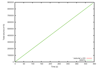
which confirms that everything works as expected.
Time-dependent inflow
The flow we have defined is constant at 2000 cumecs. What if we want to define a time-dependent flow? If we look at the syntax reference for DischargeElevation, we find that the constant value of 2000 we specified is actually a particular case of GfsFunction. We can then replace it with any of the other forms a GfsFunction can take. For example:
DischargeElevation E (2000*MIN(1,t/3600)) (y > 5431400 ? 0 : -1000)
would define a flow ramping up linearly over one hour (3600 seconds) before saturating at 2000 cumecs.
In the case of the Karamea flood, the flow is not an analytical function but is given by the flow.asc file:
% more flow.asc
0.00	151.5
1.00	176.63
2.00	463.7
...
The simplest way to use this file to define the value of the flow is to use the Cartesian Grid Data (CGD) file format for the GfsFunction. We first need to convert this file to the CGD file format.
The file will only have one dimension (time). We also need the number of data points contained in the flow.asc file. This is easily obtained using:
% wc -l flow.asc
25 flow.asc
(type wc --help or man wc to learn more about the wc command). Now open your text editor and type
1 t
25
and save the file as flow.cgd. We now need to add the values for the time coordinate. Because we chose to use seconds as our time unit, these times need to be specified in seconds. We can easily extract and convert the times in the flow.asc file using the following awk script
% awk 'BEGIN{ ORS=" " }{ print $1*3600. }END{ print "\n" }' < flow.asc >> flow.cgd
The flow.cgd file now looks like
% more flow.cgd
1 t
25
0 3600 7200 10800 14400 18000 21600 25200 28800 32400 36000 39600 43200...
We now need to append the values of the flow rate (in cumecs), which can be done using
% awk '{ print $2 }' < flow.asc >> flow.cgd
The file is now ready to use. Following the documentation we can just replace the DischargeElevation line in karamea.gfs with
DischargeElevation E flow.cgd (y > 5431400 ? 0 : -1000)
and check that everything works using
% gerris2D karamea.gfs | gfsview2D flow.gfv
Adding friction
The simulation we have set up so far does not include any model for bottom friction. The friction term is of course essential for river flows as it ultimately controls the relationship between flow rate and pressure gradient (slope). Gerris does not come with predefined friction models (although it could) but rather provides several generic objects which allow a simple implementation of a wide range of friction models.
We will see how to implement the "Smart, Duncan and Walsh (2002)" (SDW) friction model. To do this, we need to add a "source" term (or more correctly a "sink" term) to each of the components of the flux (variables U and V in Gerris). This can easily be done within Gerris using the GfsSource object and its descendants. For example
Source U 1
Source V 1
would add a constant source term (with units: [units of U]/[unit of time]) to both components of the flux. Of course in the case of a friction model, the source term is not constant but depends on: the fluid velocity (or flux U, V), the water depth (P) and the "hydraulic roughness" of the bed (Z0). Gerris provides an object - descendant of GfsSource - which is specialised for the definition of source terms applied to a velocity (or flux) field, and which depend on the velocity field itself. This object implements specific integration routines which guarantee the stability of such "self-dependent" source terms. The main application of this object is the integration of Coriolis force source terms, for example
SourceCoriolis 1e-4
is equivalent to
Source U -1e-4*V
Source V 1e-4*U
(but uses a robust integration scheme). 1e-4 is the value (units of 1/[unit of time]) of the Coriolis coefficient. We see that a general friction term will have a form which can be expressed (in Gerris syntax) as
Source U -f(U,V,P,Z0)*U
Source V -f(U,V,P,Z0)*V
which is similar to the Coriolis force. A natural extension of the SourceCoriolis syntax is then
SourceCoriolis 0 f(U,V,P,Z0)
where the Coriolis coefficient is now zero and the additional "friction coefficient" is given by the friction model. In the case of the SDW friction model, this friction coefficient is given by
<math> f(U,V,P,Z0)={\sqrt{U^2+V^2}\over P^2r^2} </math>
with <math>r=5\,(\log(a) - 1 + 1.359/a)/2</math> if <math>a<e</math>, <math>r=0.46\,a</math> if <math>a\geq e</math> and <math>a=P/Z0</math>. Using the C syntax of Gerris, this can be written in the parameter file as
SourceCoriolis 0 {
    /* r = U/U^\star */
    double Z0 = 0.01; /* 10 mm */
    if (P < 1e-6 || Z0 < 1e-6)
      return 1e10;
    double a = P/Z0;
    double r = a > 2.718 ? 2.5*(log (a) - 1. + 1.359/a) :
               0.46*a;
    return sqrt(U*U+V*V)/(P*P*r*r);
}
where care has been taken to avoid division by zero. Note also that for now we have fixed the hydraulic roughness to a constant of 0.01 metres.
Variable hydraulic roughness
To use a variable hydraulic roughness we just need to define a new variable Z0 initialised with some roughness data. I will assume that the roughness was deduced from post-processing of lidar "hits" and that the result is contained in an ASCII, compressed file called Z0.txt.gz. The file looks like this:
% zcat Z0.txt.gz | more
1533443.88,5433375.97,  18.88,0.0032
1533443.85,5433375.06,  18.87,0.0032
1533443.79,5433373.24,  18.77,0.0032
...
where the first two columns are the coordinates (in the same coordinate system as the topography topo.asc), the third column is the elevation and the last column is the roughness length scale (in metres). We can import this dataset using a technique similar to what we used to import the topography file topo.asc. We first need to create a "terrain" database using as before the xyz2kdt command, combined with awk to convert the file to the correct format. The following command will do just this
% zcat Z0.txt.gz | \
  awk 'BEGIN{FS=","}{ if ($4 > 0.) print $1, $2, $4; }' | \
  xyz2kdt -v z0
Note that we have redefined the FS variable of awk, so that fields are separated by commas rather than spaces.
Once the new terrain database has been created, we can initialise the corresponding variable by adding
VariableTerrain Z0 { basename = z0 }
in the karamea.gfs file. This line needs to be added before the line where we use the Z0 variable in SourceCoriolis.
Note that VariableTerrain is an object we have not used before. The main difference with RefineTerrain is that this object only defines a single variable (the average value of the terrain) and does not modify the mesh. Furthermore this object also updates the value of the variable whenever the mesh changes (always using the highest-possible resolution available in the corresponding terrain database). We will see later that this is useful when using adaptive mesh refinement.
For now, let's try to run our modified karamea.gfs simulation. If we do
% gerris2D karamea.gfs | gfsview2D flow.gfv
we get the following message from Gerris
gerris: file `karamea.gfs' is not a valid simulation file
karamea.16:22: error compiling expression
 In function `f':
18: error: redeclaration of `Z0'
/tmp/gfsx9MabT:12: error: `Z0' previously declared here

gfsview: <stdin>: Broken pipe
Error messages in Gerris almost always contain a line starting with something like karamea.16:22:.... The first part is the name of the file which contains the error, the first number is the line in this file at which the error occured and the second number is the column at which the error occured. Any decent text editor should allow you to navigate quickly to this line/column position in the karamea.gfs file. If you do this, you will see that the error occured when reading the GfsFunction part of the line starting with SourceCoriolis. The next lines in the message tell you more precisely what the problem is i.e.
18: error: redeclaration of `Z0'
at line 18 in the parameter file. Gerris complains about the inconsistency of defining a new variable Z0 (with the VariableTerrain line we have added) and then trying to use another (constant) variable with the same name. Fixing the problem is simple, just remove the line
double Z0 = 0.01; /* 10 mm */
and Gerris will use the new Z0 variable as should be.
It is a good idea to check that the value of Z0 is indeed correct. We can easily do this using
% gerris2D karamea.gfs | gfsview2D
and displaying Z0 using e.g. the "Squares" object in GfsView. We get

which looks consistent with our dataset i.e. a minimum roughness of 2 mm and a maximum of 0.5 metre.
Using adaptivity
So far we have only used static mesh refinement, not true adaptivity where the resolution continually changes to appropriately resolve the solution as it evolves. The goal is of course to reduce the total number of grid points and thus the total runtime.
For the case of river flows, a first simple use of adaptivity is to only refine the mesh where there is water. The dry terrain will use the coarsest possible resolution. This can be done by adding
AdaptFunction { istep = 1 } { cmax = 0 maxlevel = 8 } (P > 0)
to the parameter file. This tells Gerris to adapt the mesh at every timestep ({ istep = 1 }) using a maximum of 8 levels of refinement (maxlevel = 8). The mesh will be refined whenever the cost function (P > 0) is larger than cmax. Here we use the C convention that (P > 0) is equal to one whenever P (the water depth) is larger than zero and is equal to zero otherwise. We see that this forces Gerris to refine to eight levels of refinement whenever the flow depth is larger than zero.
If we now run the modified simulation
% gerris2D karamea.gfs | gfsview2D flow.gfv
and select "Cells" in GfsView to visualise the mesh, we get something like this
wich doesn't look good. What is happening?
We first see that the mesh is refined - as it should - only for the wet terrain, however the water depth does not look right: the riverbed is too wide. This is even more obvious if we display Zb (the topographic height) rather than P.
The problem is that by default Gerris initialises the values of variables (including Zb) by linearly interpolating the coarser mesh values. This is appropriate in most cases (i.e. when the value of the variable is part of the solution being sought). The topography Zb is not part of the solution however. What we need is an initialisation procedure which always uses the finest-scale topography data to define values of Zb in the new cells being created. This is exactly what the GfsVariableTerrain object we have introduced before does.
To use it we need to replace
RefineTerrain 8 T { basename = topo } (Te > 0.1)
with
Refine 8
VariableTerrain Zb { basename = topo }
The first line will create an (initial) uniform mesh with 8 levels of refinement and the second line will ensure that Zb is always defined using the finest relevant data in the topo terrain database. We also need to remove
Init {} { Zb = T0 }
since this was only relevant when RefineTerrain was used.
If we now run the simulation again
% gerris2D karamea.gfs | gfsview2D flow.gfv
we get something like
which looks definitely better. The simulation is also significantly faster than when using only static mesh refinement.
You may have noticed that the first few timesteps are much slower than subsequent ones. This is because we have defined an uniformly-refined initial mesh. The simulation starts with 256 x 256 cells, the vast majority of which cover dry terrain. Over the first few timesteps this number is quickly reduced to just a few hundred cells (concentrated in the "wet" inflow close to the right-hand-side boundary). Although this initially-slow calculation is not a big issue when compared with the total runtime of the simulation, the memory usage associated with the initial mesh could be an issue (not really for a 256 x 256 mesh but will become if we increase the maximum resolution). We can improve this by replacing
Refine 8
with
Refine 5
Refine (x > 1529380 && y > 5431460 && y < 5431560 ? 8 : 5)
The first line defines a 32 x 32 uniform grid. In the second line, we have used a function which uses the C conditional operator to define a level of refinement of 8 within the inflow area and 5 elsewhere.
Better adaptivity
At the moment we only adapt the mesh to a constant (maximum) resolution in wet areas. We can do better by only refining the mesh in the wet areas where it is "necessary" to resolve small-scale details. Of course the definition of "necessary" depends on many considerations and the "optimal" criterion (or combination of criteria) can only be found after experimentation. For flooding simulations, a critical aspect is that some areas such as stop-banks need to be sufficiently resolved to act as proper barriers to the flow in the simulation. This can be ensured using for example the following adaptation criterion
AdaptFunction { istep = 1 } {
    cmax = 0
    minlevel = (t > 0 ? 0 : 8)
    maxlevel = 11
} (P > 0 && Zbn > 1 ? MAX(Zbdmax - H, 0) : 0)
where Zbn and Zbdmax are defined by VariableTerrain. This is similar to the criterion we have used before. First of all we have added the condition Zbn > 1 i.e. we will refine the mesh only if it is coarse enough to contain at least
two terrain database samples. If both conditions are verified, the cost of adaptation is set to Zbdmax - H if this is positive or zero otherwise. As described in the VariableTerrain documentation, Zbdmax is the maximum elevation of any database sample contained within the cell. H is the water elevation, so that the cost function is the maximum height above the local water level of any database sample. We set cmax to zero, so we will adapt to the maximum resolution (maxlevel = 11) whenever a wet cell contains at least one "dry" sample.
If we now restart the simulation using this criterion instead of the previous one, we get something looking like
i.e. the mesh is adaptively refined to follow the "water's edge" at the highest resolution. Flooded areas are resolved at the coarsest possible resolution.
How much did we "gain" by using this criterion compared to, say, using a constant resolution? We can use OutputBalance to find out. Adding
OutputBalance { istep = 10 } stderr
to the simulation file will outputs lines looking like
Balance summary: 1 PE
  domain   min:      2254 avg:      2254         |       0 max:      2254
which tells you that you are running on a single processor (1 PE) and that the simulation contains 2254 cells. This number can be compared to the number of cells of a constant-resolution domain with the same maximum resolution i.e. 2^11^2 = 2^22 ~ 4.2 million.
Tidal boundary conditions
As you may have noticed if you know the area around Karamea, for the moment the "sea" is empty in our model. Before we look at tides, we need to fill the sea in. By default all variables in Gerris are set to zero at initialisation. This includes the depth P which is why the domain is initially dry in our simulation. To fill the sea, assuming that the sealevel is at Zb = 0, we need to set the initial fluid depth so that the water level P + Zb is equal to zero when Zb is negative. This is easily done using
Init {} {
     P = MAX(-Zb, 0)
}
i.e. P is zero (dry) when Zb is positive and the water level P + Zb is equal to zero when Zb is negative.
For simplicity, we will impose tidal boundary conditions only on the left-hand-side boundary of the domain. To start with, we will assume that the sealevel on this boundary is given by
<math> H(t) = A\sin(2\pi t/T_0) </math>
where <math>A</math> is the tidal amplitude (say 1 metre) and <math>T_0</math> is the tidal period (433512 seconds for the M2 tide). We can impose this water level on the left-hand-side boundary using
...
left = Boundary {
    BcSubcritical U MAX(1.*sin(2.*M_PI*t/433512.) - Zb, 0)
}
...
Note that the first argument of BcSubcritical must be the component of the flux normal to the boundary (U for left/right and V for top/bottom). The second argument specifies the water depth we want to impose (not the water level), so we have used the same trick as used previously for the inflow condition.
The GfsRiver solver also requires explicit boundary conditions on the top and bottom boundaries (which are now wet). We can use the default symmetry conditions of GfsBoundary (i.e. normal velocity/flux is zero on the boundary, all other quantities are symmetrical). Altogether this gives the following conditions:
GfsBox {
    right = Boundary {
	BcDirichlet P (y > 5431400 ? MAX(E - Zb, 0) : -1000)
    }
    left = Boundary {
        BcSubcritical U MAX(1.*sin(2.*M_PI*t/433512.) - Zb, 0)
    }
    top = Boundary
    bottom = Boundary
}
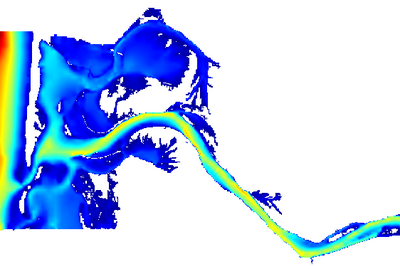
If we now restart the simulation, we can check that the sea (and branches of the estuary) are indeed filled in
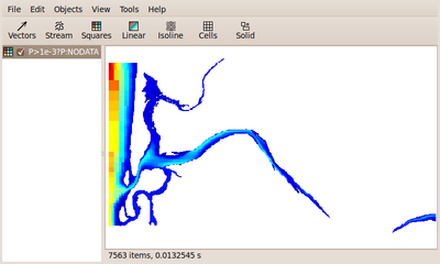
Of course refining the sea/land transition according to our adaptive refinement criterion requires more cells as indicated by the code output
...
Balance summary: 1 PE
  domain   min:     32764 avg:     32764         |       0 max:     32764
...
and the runtime is noticeably larger.
Importing the results into a GIS application
The simplest way to import the results into a GIS application is to convert them into a gridded (or raster) dataset. Using a regular grid rather than the adaptive quadtree mesh will result in (much) larger files but GIS systems are usually designed to be able to deal with large raster datasets. A standard GIS raster file format is the ESRI grid ASCII format (which we used as input for the terrain). The GfsOutputGRD Gerris object can be used to export fields using this format. For example
OutputGRD { step = 600 } p-%g.asc { v = P }
will create files called: p-0.asc, p-600.asc, p-1200.asc, ... (at 10 minutes intervals) which describe the evolution of the fluid depth P. These files can be imported directly into a GIS application.
Optimising the simulation
There are several things we can do to optimise the simulation.
By default GfsRiver uses a second-order time integration scheme. This is important for phenomena which have physical time scales comparable to the integration timestep (e.g. tsunamis). Using first-order-in-time schemes for such phenomena would lead to excessive numerical damping. In our river flood case, we saw that the timestep required for stability (at the maximum resolution we used) is around 0.2 seconds. This is much shorter than any (transient) phenomena we are interested in (indeed if we are interested only in the stationary regime then there is no physical timescale at all), so that we can safely use the first-order time integration scheme. Following the GfsRiver manual, this is done simply by adding
} {
    time_order = 1
}
in the right spot. This should speed up the run by up to a factor of two.
Another parameter which is worth controlling is the water level below which the terrain is considered "dry", By default this is set to <math>10^{-6}</math> times the size of the box i.e. in our case: <math>10^{-6}\times 5600=5.6</math> millimetres. To be consistent, we should use this value, rather than zero whenever we need to distinguish "wet" from "dry" cells. It is simplest to do this by defining a text macro using
Define DRY 1e-3
and use it where we need the depth of dry cells, for example:
SourceCoriolis 0 {
    /* r = U/U^\star */
    if (P < DRY || Z0 < 1e-6)
        return 1e10;
    double a = P/Z0;
    double r = a > 2.718 ? 2.5*(log (a) - 1. + 1.359/a) :
               0.46*a;
    return sqrt(U*U+V*V)/(P*P*r*r);
}
Because we chose a value different from the default of 5.6 mm, we also need to tell GfsRiver to use it, which can be done with
} {
    time_order = 1
    dry = DRY
}
Epilogue
The final simulation file
If you have followed the tutorial, you should end up with something close to the following
Define DRY 1e-3

1 0 GfsRiver GfsBox GfsGEdge { x = 0.5 y = 0.5 } {
    PhysicalParams { L = 5600 g = 9.81 }
    MapTransform { tx = 1523880 ty = 5430180 }
    GModule terrain
    Refine 8
    VariableTerrain Zb { basename = topo }
    VariableTerrain Z0 { basename = z0 }
    SourceCoriolis 0 {
	/* r = U/U^\star */
	if (P < DRY || Z0 < 1e-6)
	    return 1e10;
	double a = P/Z0;
	double r = a > 2.718 ? 2.5*(log (a) - 1. + 1.359/a) :
                   0.46*a;
	return sqrt(U*U+V*V)/(P*P*r*r);
    }
    Init {} {
	P = MAX(-Zb, 0)
    }
    DischargeElevation E flow.cgd (y > 5431400 ? 0 : -1000)
    AdaptFunction { istep = 1 } {
	cmax = 0
	minlevel = (t > 0 ? 0 : 8)
	maxlevel = 11
    } (P > DRY && Zbn > 1 ? MAX(Zbdmax - H, 0) : 0)
    OutputTime { istep = 10 } stderr
    OutputBalance { istep = 10 } stderr
    OutputSimulation { step = 10 } stdout
    OutputScalarSum { istep = 10 } volume { v = P }
} {
    time_order = 1
    dry = DRY
}
GfsBox {
    right = Boundary {
	BcDirichlet P (y > 5431400 ? MAX(E - Zb, 0) : -1000)
    }
    left = Boundary {
	BcSubcritical U MAX(1.*sin(2.*M_PI*t/433512.) - Zb, 0)
    }
    top = Boundary
    bottom = Boundary
}
which you can run using
% gerris2D -m karamea.gfs | gfsview2D flow.gfv
Alternative way of imposing inflow conditions
GfsDischargeElevation can only be used where the river channel intersects a boundary of the simulation domain. It is sometimes useful to be able to impose an inflow in the middle of the domain (i.e. a "spring"). This can be done using the GfsSourceFlux object of Gerris. The following describes how to use GfsSourceFlux to impose an inflow condition.
Reading the documentation, we find that aside from the flow value we need to define the area on which the flow will be imposed. This area is defined using a function of the spatial coordinates (x and y) of our simulation domain.
We could work out what this function is using geographical coordinates, however for this particular example it is simpler to just visualise the terrain and construct this function interactively using GfsView. To do this we can use the end.gfs simulation we generated above and visualise it using GfsView:
% gfsview2D end.gfs isolines.gfv
We want to impose the inflow close to the right-hand-side boundary of the domain. Pan and zoom to display this part of the domain, then select "Objects -> Mesh -> Boundaries", click on "Squares", change "P" to "T0" and you should get something looking like this
which shows the right-hand-side boundary together with the upper reaches of the river. We now want to define a rectangular box within which to impose the inflow. To find the value of the left-hand-side (or lower value) x-coordinate of this box, hold the "Ctrl" key of your keyboard while clicking on the left mouse button. The coordinates of the mouse cursor are then displayed in the status bar of GfsView (see screenshot above): a lower x-coordinate value of 1529380 seems appropriate. To test whether this is OK, replace "T0" in the "Scalar" text entry of the "Squares" property dialog with "x > 1529380" and you will get
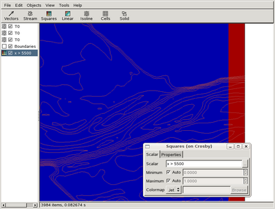
i.e. we have defined a band along the right-hand-side boundary. We would like to restrict this band vertically to coincide with the river bed. Using the "Ctrl-click" technique we find that values of the y-coordinate between 5431460 and 5431560 are appropriate. To test this replace "x > 1529380" with
(x > 1529380 && y > 5431460 && y < 5431560)
where "&&" is the logical "AND" operator in C. This will give something like
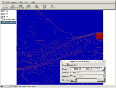
which gives a visual check that everything is OK. We could also adjust the box coordinates by directly editing the values in the formula above. Note also that we are not restricted to square boxes, any function can be used so that almost any shape can be generated (for example we could use the function for the township refinement above to define a circular inflow area).
This function can now be used in GfsSourceFlux as:
SourceFlux P 2000 (x > 1529380 && y > 5431460 && y < 5431560)
Adding culverts
From a modelling point of view culverts are a coupled sink and source of mass and/or momentum. They are modelled as segments connecting two discretisation cells. The flow rate between these two cells is then controlled by a "culvert model" which takes as input the water depths and momentum at either ends of the segment, any intrinsic properties of the culvert (e.g. length, width, height, roughness etc.) and returns the flow rate.
We will consider as an example an underground pipe connecting either sides of a road embankment in the Karamea terrain model. To start with we will consider a flooding scenario without the pipe. We will start from the previous file but at a coarser resolution to speed things up. Open the karamea.gfs file and replace the lines
DischargeElevation E flow.cgd (y > 5431400 ? 0 : -1000)
...
maxlevel = 11
with
DischargeElevation E 1500 (y > 5431400 ? 0 : -1000)
...
maxlevel = 9
Then rerun the simulation with
% gerris2D -m karamea.gfs | gfsview2D flow.gfv
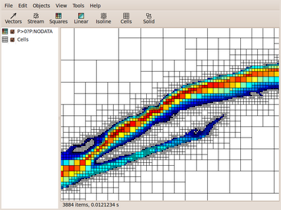
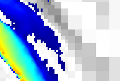
Wait until the simulation has run to a bit more than four hours simulated time and, playing with the parameters of GfsView, you should be able to get a figure looking like this (tip: use P > 1e-3 ? P : NODATA as scalar value)
Adding the bathymetry (Zb) with a grayscale and zooming on the center of the image reveals that a flooded branch is contained by an embankment: the light band between water and a deeper (darker) valley on the right-hand-side in the image below
What would happen if a culvert traversed the embankment at this location? We first need to find the coordinates of both ends of the culvert. We can do this for example by Ctrl-clicking on the GfsView display (in a more realistic scenario the culvert geographic coordinates would of course be given from e.g. field data). This gives for our example the following pair of coordinates
(1526896,5432714) (1526922,5432735)
Rather than rerun the simulation from the start after adding the culvert, we will restart the simulation from where we are at. We can save the state of the simulation from GfsView (an alternative would have been to save the state of the simulation at regular intervals using GfsOutputSimulation in the parameter file). Click on the File -> Save menu in GfsView (or type Ctrl-S) and type snapshot.gfs in the 'Path' dialog, then click on the 'Save' button. You can now stop the simulation using either Ctrl-C in the terminal where you started it or using the File -> Quit menu (Ctrl-Q) in GfsView. If you now reopen the saved snapshot using
% gfsview2D snapshot.gfs
you should recover the same visualisation. If you now open snapshot.gfs with a text editor, you will see that it looks like (and is) a regular parameter file. To add the culvert just add
SourcePipe *culvert (1526896,5432714) (1526922,5432735) 2
for example before the GfsDischargeElevation line. The parameters are in order: a symbolic name (optional), the coordinates of both ends of the culvert and the pipe diameter (in metres). Have a look at the documentation of GfsSourcePipe for details. To check that the culvert is correctly defined, save the file and reopen it with GfsView
% gfsview2D snapshot.gfs
then select the Objects -> Special -> Pipes menu. Zooming in you should see
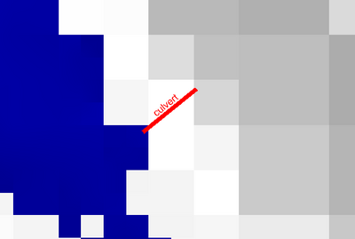
The length and width of the red rectangle match the end points and diameter given in the parameter file. You can now restart the simulation using
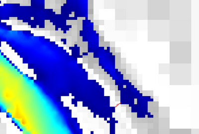
% gerris2D snapshot.gfs | gfsview2D flow.gfv
After about 7 hours of simulated time, the valley on the right-hand-side of the embankment is now flooded by water flowing through the culvert
More realistic culverts can be modelled using the culvert module.
References
- Syntax reference for Gerris.
- Gerris terrain databases at NIWA.
- Relatively rough flow resistance equations Graeme M. Smart; Maurice J. Duncan; and Jeremy M. Walsh - JOURNAL OF HYDRAULIC ENGINEERING, 2002, 568-578. PDF
