From Gerris

Contents 1 Very very simple tutorial 2 Gerris as a language 2.1 Sample code: box 2.2 Sample code: boundary condition for a box 2.2.1 Example of Boundary conditions 2.3 Sample code: first try 2.4 Sample code : intermezzo 2.5 Sample code : second try 2.6 Sample code: viscosity 2.7 Sample code : third try 2.8 Sample code : fourth try 2.9 Sample code: adding a box 3 Gfsview: a graphical tool 4 Adding objects 4.1 Wake behind a cylinder 5 Adaptive meshing 6 Passive tracer and Adaptive meshing 7 (Less) passive tracer: VOF technique 7.1 Adding surface tension 7.2 Breaking bubbles 8 Gerris in parallel

Very very simple tutorial

This is a step by step tutorial to Gerris.

Gerris is a Partial Differential Equations Solver (PDES) for the time-dependent incompressible variable-density Euler, Stokes or Navier-Stokes equations (and some variants). Gerris is also a programming language and we begin now with some basic concepts.

Gerris as a language

When we learn a language we begin with words, then syntax, and then semantic.

The Gerris language is composed by words that reflect the internal structure of the code. The Gerris code is written in C with inheritance.

The Gerris language is an inheritance language where the root of each word is a component of its parent.

For example

• GfsOutputTiming (write summary of time consumption of the simulation)
• GfsOutputTime (write the model time, timestep, CPU time and real time)
• GfsOutputSimulation (write the whole simulation data)

have the same parent GfsOutput which write simulation data. If we understand the inheritance we make a big step forward.

In practice we write a code on a script line by line following the Gerris syntax and the Gerris solver interprets it.

Sample code: box

Simplest Gerris code doing nothing!!!

1 0 GfsSimulation GfsBox GfsGEdge {} {
  Refine 5
  # Code Gerris here!!
OutputSimulation { step = 1 } stdout 
}
GfsBox {
  # Boundary conditions here!!
}

Gerris uses a box of length L=1 (in 2D) or a cube (in 3D) to build a domain, in this case we use the 2D solver. We have

1 0 GfsSimulation GfsBox GfsGEdge {} {

1 0 says one box (1) not connected (0) and the other words (GfsSimulation GfsBox GfsGEdge) are Gerris reserved words.

The line

Refine 5

gives us the initial mesh, we have created a regular Cartesian grid with 2*2*2*2*2=32 cells in each dimension. We can use this Gerris keyword to refine the initial mesh.

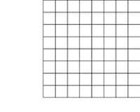
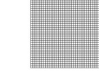
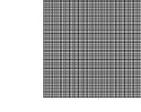
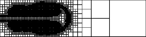
The Figures show the mesh for Refine 3, Refine 5 and Refine 6. We can use every C expression, for example

Refine (y < x ? 6 : 3)

which gives Refine 6 for y < x and Refine 3 for y > x

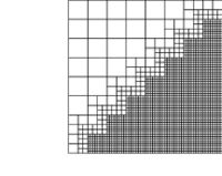
The Figure shows two important things about the structure of Gerris

1. y = x pass through the center of the box so that the origin (0,0) is at
2. the center of the box!! (Tip you can displace the origin using)
3. We pass every mesh level one by one

Finally

GfsBox {
  # Boundary conditions here!!
}

allows to impose the Boundary conditions for our only box. Note that you must repeat the GfsBox structure for as many boxes as indicated in the first line.

Sample code: boundary condition for a box

A box has 4 sides (top, bottom, left and right). The Gerris language uses these key words to impose the boundary conditions.

By default Gerris assumes that boundaries are solid walls with slip conditions for the velocity, we then have defined a rectangular box closed on all sides by solid walls.

Gerris uses two families of words: GfsBoundary and GfsBc, with the corresponding inheritances.

GfsBoundary is used to define boundary conditions on the boundaries for the box with the following syntax

GfsBoundary {
  [ GfsBc ]
  [ GfsBc ]
}

where [ GfsBc ] are one of the descendants

• GfsBcDirichlet — Dirichlet boundary condition (i.e. value)
• GfsBcNeumann — Neumann boundary condition (i.e. value of the normal derivative)
• GfsBcNavier — Navier slip/Robin boundary condition

We note that GfsBoundary have also two particular descendants

• GfsBoundaryInflowConstant — Constant inflow
• GfsBoundaryOutflow — Free outflow/inflow

Example of Boundary conditions

Velocity U=1 at the left and outflow condition at the right

GfsBox {
  left = Boundary {
    BcDirichlet U 1
  }
  right = BoundaryOutflow
}

Pressure P=1 at the left pressure P=0 at the right

GfsBox {
  left = Boundary {
    BcDirichlet P 1
  }
  right =  Boundary {
    BcDirichlet P 0
  }
}

We note that we can use here: U, V, P as variables and every C function (including time t and space x and y) like

GfsBox {
  left = Boundary {
    BcDirichlet U ( sin(2.*M_PI*0.05*t) )
  }
  right = BoundaryOutflow
}

a sinusoidal velocity at the left side and an outflow condition at the right side.

Sample code: first try

We can build now a simulation file for a box of length L=1, with a mesh of 32x32 (Refine 5) and with an input velocity equal to 1.

1 0 GfsSimulation GfsBox GfsGEdge {} {
  Refine 5
}
GfsBox {
  left = Boundary {
    BcDirichlet U 1
  }
  right =  BoundaryOutflow
}

We save the file as tutorial1.gfs and a console we run the simulation

gerris2D tutorial1.gfs

and nothing happens.

Sample code : intermezzo

We need to define the computational time and the data we want to output.

The Gerris word GfsTime defines the physical and the computational time (number of time steps performed). By default both the physical time and the time step number are zero when the program starts. It is possible to set different values using for example

GfsTime { t = 1.4 i = 32 }

where i is the time step number and t is the physical time. The end identifier specifies that the simulation should stop when the physical time reaches the given value. It is also possible to stop the simulation when a specified number of time steps is reached, using the iend identifier. If both end and iend are specified, the simulation stops when either of these are reached. By default, both end and iend values are infinite.

GfsTime { end = 2 iend = 32 }

Gerris comes with a number of objects allowing to output specific data of the simulation. For that we need take a look at GfsOutput. A generic object which defines a given family (parent and childrens).

The parent of GfsOutput is GfsEvent which is used to control any action which needs to be performed at a given time during a simulation. The keywords for GfsEvent are

start

Physical starting time (default is zero). The "end" keyword can be used to indicate the end of the simulation.

istart

Time step starting time (default is zero).

step

Repeat every step physical time units (default is infinity).

istep

Repeat every istep time steps (default is infinity).

end

Stop at or before this physical time (default is infinity).

iend

Stop at or before this number of time steps (default is infinity).

The children of GfsOutput are .. many ... (a rabbit family). Here are a few

• GfsOutputSimulation which writes the whole simulation. The syntax is

 GfsOutputSimulation {inheritance of GfsOutput, then of GfsEvent}

For example

 GfsOutputSimulation { start = 0.6 step = 0.3 } file.gfs

which says, we write into a file file.gfs every 0.3 of physical time starting from 0.6. The data format gfs is a Gerris format and we will talk about it later. Note that you can save data in other formats if you want.

• GfsOutputLocation which write the values of variables at specified locations

the syntax is

 GfsOutputLocation {inheritance of GfsOutput, then of

GfsEvent} positionXYZ For example

 GfsOutputLocation { step = 1 } data positionXYZ

which says do every unit time the following: write in file data the numerical values of the dynamical variables at positions given by the input file positionXYZ. The input file is an ascii file with three columns of coordinates (x y z)

0 -0.5 0 
0 -0.49 0 
0 -0.48 0
0 -0.47 0
0 -0.46 0
0 -0.45 0
......
0 0.44 0
0 0.45 0
0 0.46 0
0 0.47 0
0 0.48 0
0 0.49 0
0 0.5 0

Generating such a file 'by hand' using your favorite text editor can be tedious. But the following script will do the job:

 (for ((a=-50; a <= 50 ; a++)); do echo 0 `echo $a | awk '{print $1/100.}'` 0; done) > positionXYZ

Sample code : second try

Finally we do the second try

1 0 GfsSimulation GfsBox GfsGEdge {} {
  Refine 5
  GfsTime { end = 5 }
  GfsOutputLocation { step = 1 } data positionXYZ
}
GfsBox {
  left = Boundary {
    BcDirichlet U 1
  }
  right =  BoundaryOutflow
}

this Gerris script does the following:

1. it stops the run at physical time 5 GfsTime { end = 5 } ,
2. writes the results into the file data at the positions given by the
3. file positionXYZ,
4. the boundary conditions are an imposed pressure at both ends

We save the file as tutorial2.gfs and in a console we run the simulation

gerris2D tutorial2.gfs

and something happen but it seems strange... U = 1 everywhere, what's wrong?

Sample code: viscosity

We forgot the viscosity!!! we take now take a look at the Gerris documentation

By default, the density is unity and the molecular viscosity is zero (i.e. there is no explicit viscous term in the momentum equation). In practice, it does not mean that there is no viscosity at all however, because any discretization scheme always has some numerical viscosity. However, keep in mind that the only relevant parameter for the (constant density) Navier-Stokes equations is the Reynolds number. If you do not include any explicit viscous term the (theoretical) Reynolds number is always infinite.

So our script is wrong, good syntax but bad semantic!!! That tels us that we have to think about the physical problem first!!!

We need to set the viscosity, GfsSourceViscosity can do it

GfsSourceViscosity  'value or function'

for instance if we decide to do the simulation in dimensionless variables (the good procedure) we can set the viscosity as 1/Re where Re is the Reynolds number

GfsSourceViscosity  1.

where the Reynolds number is now 1.

Sample code : third try

We write now

1 0 GfsSimulation GfsBox GfsGEdge {} {
  Refine 5
  GfsTime { end = 5 }
  GfsSourceViscosity  1
  GfsOutputLocation { step = 1 } data positionXYZ
}
GfsBox {
  left = Boundary {
    BcDirichlet U 1
  }
  right = BoundaryOutflow
}

this Gerris script does the following :

1. it stops the run at 5 physical times GfsTime { end = 5 } ,
2. sets the Reynolds number to 1.
3. writes the results into the file data at the positions given by the file positionXYZ,
4. the boundary conditions are imposed pressure at both ends

We save the file as tutorial3.gfs and a console we run the simulation

gerris2D tutorial3.gfs

and it works!!

We take a look at the file data, there are several columns and the first line gives the label of each column

 # 1:t 2:x 3:y 4:z 5:P 6:Pmac 7:U 8:V

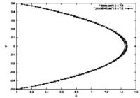
Using gnuplot (plot [0:2] "./data.dat" i 5 u 7:3 w lp) we can do a graph of the final time (t=5)

and the velocity U is constant!!! Where is our classical parabolic profile??

Sample code : fourth try

We now set all boundary conditions (top and bottom are set to zero). We also add an "OutputTime" command to have something to look at during the run.

1 0 GfsSimulation GfsBox GfsGEdge {} {
  Refine 5
  Time {end = 5}
  SourceViscosity 1.
  OutputLocation { start = end } data.dat positionXYZ
  OutputSimulation { step = 1 } tt.gfs
  OutputTime { step = 1 } stdout
}
GfsBox {
  left = Boundary {
    BcDirichlet U 1
  }
  right =  BoundaryOutflow
  top  =  Boundary {
    BcDirichlet U 0
    BcDirichlet V 0
  }
  bottom = Boundary {
    BcDirichlet U 0
    BcDirichlet V 0
  }
}

We save the file as tutorial4.gfs and in a console we run the simulation

gerris2D tutorial4.gfs

and using

 gnuplot -e 'plot "./data.dat" u 7:3 w lp'

we get a graph of the final time

It is better but, as we shall see it is not exactly the expected parabolic profile.

Indeed we can look near the exit at coordinates (x = 0.45), recall that domain is [-0.5:0.5].

Using awk we modify the file positionXYZ to translate it towards the outflow boundary

awk '{print $1+0.45 " " $2 " " $3 }' positionXYZ > positionX0.45YZ

and we now write

1 0 GfsSimulation GfsBox GfsGEdge {} {
  Refine 5
  Time {end = 5}
  SourceViscosity 1.
  OutputLocation { step = 1 } data positionXYZ
  OutputLocation { step = 1 } data0.45 positionX0.45YZ
}
GfsBox {
  left = Boundary {
    BcDirichlet U 1
  }
  right = BoundaryOutflow
  top  = Boundary {
    BcDirichlet U 0
    BcDirichlet V 0
  }
  bottom = Boundary {
    BcDirichlet U 0
    BcDirichlet V 0
  }
}

where we generate two files data and data0.45. the results are

humm, we will add a box.

Sample code: adding a box

Now we add a box to the right of our first box (the domain is now 2x1), 2 in x coordinates [(0.5:1.5)]. We generate also a new file positionX1.45YZ to study the profile at the end of the two boxes. We modify the Gerris file as follows

2 1 GfsSimulation GfsBox GfsGEdge {} {
  Refine 5
  Time { end = 5 }
  SourceViscosity 1.
  OutputLocation { step = 1 } data positionXYZ
  OutputLocation { step = 1 } data0.45 positionX0.45YZ
  OutputLocation { step = 1 } data1.45 positionX1.45YZ
}
GfsBox {
  left = Boundary {
    BcDirichlet U 1
  }
  top  =  Boundary {
    BcDirichlet U 0
    BcDirichlet V 0
  }
  bottom  =  Boundary {
    BcDirichlet U 0
    BcDirichlet V 0
  }
}
GfsBox {
 right = BoundaryOutflow 
 top  =  Boundary {
   BcDirichlet U 0
   BcDirichlet V 0
 }
 bottom  =  Boundary {
   BcDirichlet U 0
   BcDirichlet V 0
 }
}
1 2 right

We have in the first line 2 1 which says two (2) boxes with one (1) connection, and we add two GfsBox one for each box together with the corresponding boundary conditions. The new line

1 2 right

say that the boxes 1 and 2 are connected by the right side (beginning from box 1).

Gfsview: a graphical tool

GfsView is a tool written specifically to visualize Gerris simulation files. We have seen the Gerris keyword GfsOutputSimulation before, we modify then our script adding the line

GfsOutputSimulation { start = end } file.gfs

which says write the whole simulation in file file.gfs at the final time.

Now we can run Gfsview

gfsview2D file.gfs

and clicking on “Linear”, “Vectors” in the tool-bar and changing the vector length by editing the properties of the “Vectors” object (select the object then choose “Edit→Properties”) you should be able to get something looking like

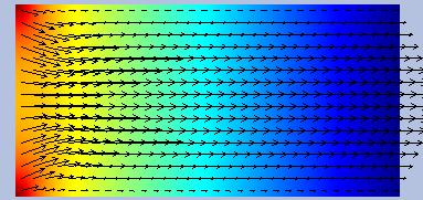
You can also pan by dragging the right mouse button, zoom by dragging the middle button and rotate by dragging the left button.

You can get the value of an object by selecting the object on the left panel; then press the Ctrl key and click on the position where you want to get the object value, while continuing to hold the Ctrl key.

If you like a given representation of results and you want to reuse it you can save the Gfsview file ("Save" in toolbar) in gfv format, like vectors.gfv. Now you can start Gfsview directly with the saved parameters

gfsview2D file.gfs vectors.gfv

We can pipe the results at every time we want directly in Gfsview, for example

GfsOutputSimulation { step = 1 } stdout

and running

gerris2D tutorial5.gfs | gfsview2D -s vectors.gfv

but stationary flows are stationary...

Adding objects

We will add a solid object in our channel, a cylinder. Gerris uses implicit functions to define solids, the Gerris keyword is GfsSolid and the syntax

GfsSolid ( implicit function )

for example, a circle of radius 0.125 at (0,0) is

Solid (x*x + y*y - 0.125*0.125)

We can also refine the solid using the Gerris keyword RefineSolid, like

RefineSolid 6

We note that Gerris can deal with arbitrarily complex solid boundaries (in gts format) embedded in the quad/octree mesh but creating polygonal surfaces is not an easy job and is explained in other tutorials. We use in this case the same Gerris word, GfsSolid mycomplexsurface.gts.

Now for our cylinder the script is

2 1 GfsSimulation GfsBox GfsGEdge {} {
  Refine 5
  Solid (x*x + y*y - 0.125*0.125)
  RefineSolid 6
  Time { end = 5 }
  SourceViscosity 1.
  OutputLocation { step = 1 } data positionXYZ
  OutputLocation { step = 1 } data0.45 positionX0.45YZ
  OutputLocation { step = 1 } data1.45 positionX1.45YZ
  OutputSimulation { start = 1.0 } file.gfs
}
GfsBox {
  left = Boundary {
    BcDirichlet P 1
  }
  top  =  Boundary {
    BcDirichlet U 0
    BcDirichlet V 0
  }
  bottom  =  Boundary {
    BcDirichlet U 0
    BcDirichlet V 0
  }
}
GfsBox {
  right =  Boundary {
    BcDirichlet P 0
  }
  top  =  Boundary {
    BcDirichlet U 0
    BcDirichlet V 0
  }
  bottom  =  Boundary {
    BcDirichlet U 0
    BcDirichlet V 0
  }
}
1 2 right

Saving the Gerris script in tutorial6.gfs and running

gerris2D tutorial6.gfs 
gfsview -s vectors.gfv file.gfs

we can (not) see the Benard-Von Karman wake.

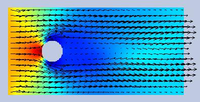
humm, let's go to a textbook...

Wake behind a cylinder

ah the Reynolds number has to be bigger than 50 and we need a long channel to allow the wake develops...

The Reynolds number is computed from the box of size 1 but for the specific case of the wake behind a cylinder the typical length is the cylinder diameter. So Red = Re/4 because the cylinder diameter is L/4.

We add also 2 other boxes (we know how) and we set the Reynolds number to 100

1. SourceViscosity 1./400.
2. the final time to 10 Time { end = 10 }
3. the final file results file10.gfs at time 10 OutputSimulation { start = end } file10.gfs

The Gerris script is

4 3 GfsSimulation GfsBox GfsGEdge {} {
  Refine 5
  Solid (x*x + y*y - 0.125*0.125)
  Time {end = 10}
  SourceViscosity 1./400.
  OutputLocation { step = 1 } data positionXYZ
  OutputLocation { step = 1 } data0.45 positionX0.45YZ
  OutputLocation { step = 1 } data1.45 positionX1.45YZ
  OutputSimulation { start = end } file10.gts 
}
GfsBox {
  left = Boundary {
    BcDirichlet U 1
  }
  top  =  Boundary {
    BcDirichlet U 0
    BcDirichlet V 0
  }
  bottom  =  Boundary {
    BcDirichlet U 0
    BcDirichlet V 0
  }
}
GfsBox {
  top  =  Boundary {
    BcDirichlet U 0
    BcDirichlet V 0
  }
  bottom  =  Boundary {
    BcDirichlet U 0
    BcDirichlet V 0
  }
}
GfsBox {
  top  =  Boundary {
    BcDirichlet U 0
    BcDirichlet V 0
  }
  bottom  =  Boundary {
    BcDirichlet U 0
    BcDirichlet V 0
  }
}
GfsBox {
  right = BoundaryOutflow
  top  =  Boundary {
    BcDirichlet U 0
    BcDirichlet V 0
  }
  bottom  =  Boundary {
    BcDirichlet U 0
    BcDirichlet V 0
  }
}
1 2 right
2 3 right
3 4 right

We find the following results

and were is the wake..? hum we will try a finer mesh, we now set

Refine 6

and now the famous wake appears!!!

conclusion: don't forget the discretization!! It could be interesting to have dynamical adaptive meshing.

Adaptive meshing

We are going to use dynamic adaptive mesh refinement, a very interesting characteristic of Gerris where the quadtree structure of the discretization is used to adaptively follow the small structures of the flow, thus concentrating the computational effort on the area where it is most needed.

This is done using GfsAdapt which inherits (again) from GfsEvent. Various criteria can be used to determine where refinement is needed. In practice, each criteria will be defined through a different object derived from GfsAdapt. If several GfsAdapt objects are specified in the same simulation file, refinement will occur whenever at least one of the criteria is verified.

GfsAdapt is the base class for all the objects used to adapt the resolution dynamically, the parameters are

minlevel

The minimum number of refinement levels (default is 0).

maxlevel

The maximum number of refinement levels (default is infinity).

mincells

The minimum number of cells in the simulation (default is 0).

maxcells

The maximum number of cells in the simulation. If this number is reached, the algorithm optimizes the distribution of the cells so that the maximum cost over all the cells is minimized (default is infinity).

cmax

The maximum cell cost allowed. If the number of cells is smaller than the maximum allowed and the cost of a cell is larger than this value, the cell will be refined.

weight

When combining several criteria, the algorithm will weight the cost of each by this value in order to compute the total cost (default is 1).

cfactor

Cells will be coarsened only if their cost is smaller than cmax/cfactor (default is 4).

We will use GfsAdaptVorticity defined as the norm of the local vorticity vector multiplied by the cell size and divided by the maximum of the velocity norm over the whole domain. The syntax is

GfsAdaptVorticity {inheritance GfsEvent} {inheritance GfsAdapt}

like that

GfsAdaptVorticity { istep = 1 } { maxlevel = 6 cmax = 1e-2 }

we can now write another Gerris script

4 3 GfsSimulation GfsBox GfsGEdge {} {
  Refine 5
  Solid (x*x + y*y - 0.125*0.125)
  Time {end = 10}
  SourceViscosity 1./400.
  AdaptVorticity { istep = 1 } { maxlevel = 6 cmax = 1e-2 }
  OutputLocation { step = 1 } data positionXYZ
  OutputLocation { step = 1 } data0.45 positionX0.45YZ
  OutputLocation { step = 1 } data1.45 positionX1.45YZ
  OutputSimulation { start = end } file10.gts 
}
GfsBox {
  left = Boundary {
    BcDirichlet U 1
  }
  top  =  Boundary {
    BcDirichlet U 0
    BcDirichlet V 0
  }
  bottom  =  Boundary {
    BcDirichlet U 0
    BcDirichlet V 0
  }
}
GfsBox {
  top  =  Boundary {
    BcDirichlet U 0
    BcDirichlet V 0
  }
  bottom  =  Boundary {
    BcDirichlet U 0
    BcDirichlet V 0
  }
}
GfsBox {
  top  =  Boundary {
    BcDirichlet U 0
    BcDirichlet V 0
  }
  bottom  =  Boundary {
    BcDirichlet U 0
    BcDirichlet V 0
  }
}
GfsBox {
  right = BoundaryOutflow
  top  =  Boundary {
    BcDirichlet U 0
    BcDirichlet V 0
  }
  bottom  =  Boundary {
    BcDirichlet U 0
    BcDirichlet V 0
  }
}
1 2 right
2 3 right
3 4 right

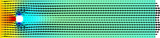
and we can look at the wake

and at the mesh distribution

Two brothers or sisters of GfsAdaptVorticity are

1. GfsAdaptGradient — Adapting cells depending on the local gradient of a variable
2. GfsAdaptFunction — Adapting cells depending on the value of a function

and you can combine them all together...

Passive tracer and Adaptive meshing

We continue to explore the adaptive meshing by the introduction of another basic concept, the passive tracer. Experimentalists use passive tracer (like ink) to visualize the fluid flows. Gerris can do that using GfsVariableTracer which advects a scalar quantity with the flow velocity, the syntax is

GfsVariableTracer tracer

For example

GfsVariableTracer T

where T is the advected (scalar) quantity. We can also use the grid refinement for the variable T

GfsAdaptGradient { istep = 1 } { maxlevel = 6 cmax = 1e-2 } T

we recognize the inheritance { istep = 1 } {maxlevel = 6 cmax = 1e-2}

We modify the boundary condition to have a thin jet of fluid at the entry and we inject the passive tracer inside,

GfsBox {
  top  =  Boundary {
    BcDirichlet U 0
    BcDirichlet V 0
  }
  bottom  =  Boundary {
    BcDirichlet U 0
    BcDirichlet V 0
  }
  left = Boundary {
    BcDirichlet U ( (y > -0.05 && y < 0.05 ) ? 1 : 0 )	   
    BcDirichlet T ( (y > -0.05 && y < 0.05 ) ? 1 : 0 )
  }
}

where ( (y > -0.05 && y < 0.05 ) ? 1 : 0 ) is a C shortcut of if variable y is between -0.05 and 0.05 set T to 1 and zero elsewhere. The new script is now

4 3 GfsSimulation GfsBox GfsGEdge {} {
  Refine 5
  Time { end = 20 }
  VariableTracer T
  SourceViscosity 1./400
  AdaptGradient { istep = 1 } {maxlevel = 6 cmax = 1e-2} T
  OutputSimulation { step = 1 } stdout
}
GfsBox {
  top  =  Boundary {
    BcDirichlet U 0
    BcDirichlet V 0
  }
  bottom  =  Boundary {
    BcDirichlet U 0
    BcDirichlet V 0
  }
  left = Boundary {
    BcDirichlet U ( (y > -0.05 && y < 0.05 ) ? 1 : 0 )	   
    BcDirichlet T ( (y > -0.05 && y < 0.05 ) ? 1 : 0 )
  }
}
GfsBox {}
GfsBox {}
GfsBox {
  right = BoundaryOutflow
}
1 2 right
2 3 right
3 4 right

where we have taken off the solid surface and the writing positions. Now we can save the file and pipe the stdout in GfsView to follow the dynamic of the entry jet

gerris2D tutorial7.gfs | gfsview2D

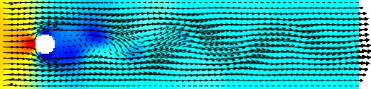
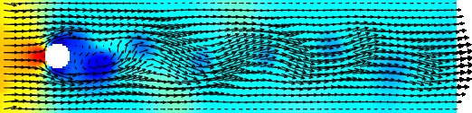
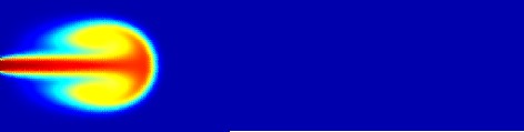
We show the velocity field and the passive tracer for two different physical times (t=1 and t=4).

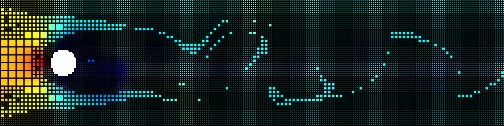
The following figure shows the mesh at different times

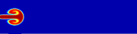
We add diffusion to the tracers using the Gerris word SourceDiffusion like so

SourceDiffusion T 0.001

and the solution for t=4 is now

we note that tracers can represent, for example, temperature or concentration.

(Less) passive tracer: VOF technique

We know that experimentalists use bubbles to analyze fluid flows (PIV). Bubbles can be a passive tracer but... can also be a field of study. Moreover every frontier separating different fluids have potential interest in academic and industry.

Gerris uses a VOF (Volume Of Fluid) technique to follow interfaces, the VOF is a numerical technique for tracking and locating interfaces, in particular fluid-fluid ones.

Gerris first defines the marker of the interface using GfsVariableTracerVOF which defines a volume-fraction field advected using the geometrical Volume-Of-Fluid technique, the syntax is

GfsVariableTracerVOF tracerVOF

The tracer will be advected and we need to define the geometrical position of the boundary. To define the frontier Gerris uses the word GfsInitFraction with the following syntax

GfsInitFraction tracerVOF (implicit surface)

We now add a bubble of radius 0.125 L (recall that L is the size of the unit box)

VariableTracerVOF T1
InitFraction T1 ((x)*(x) + y*y - 0.125*0.125)

and now our script is

4 3 GfsSimulation GfsBox GfsGEdge {} {
  Refine 5
  Time { end = 20 }
  VariableTracer T
  VariableTracerVOF T1
  InitFraction T1 ((x)*(x) + y*y - 0.125*0.125)
  SourceViscosity 1./400
  AdaptGradient { istep = 1 } { maxlevel = 7 cmax = 1e-2 } T1
  AdaptGradient { istep = 1 } {maxlevel = 6 cmax = 1e-2} T
  OutputTime { step = 1 } stderr
  OutputSimulation { step = 1 } stdout
}
GfsBox {
  top  =  Boundary {
    BcDirichlet U 0
    BcDirichlet V 0
  }
  bottom  =  Boundary {
    BcDirichlet U 0
    BcDirichlet V 0
  }
  left = Boundary {
    BcDirichlet U ( (y > -0.05 && y < 0.05 ) ? 1 : 0 )	   
    BcDirichlet T ( (y > -0.05 && y < 0.05 ) ? 1 : 0 )
  }
}
GfsBox {}
GfsBox {}
GfsBox {
  right = BoundaryOutflow
}
1 2 right
2 3 right
3 4 right

where we added mesh refinement in the line GfsAdaptGradient { istep = 1 } { maxlevel = 7 cmax = 1e-2 } T1, the following figures show the two tracers T and T1 for physical times t=1 and t=4.

Adding surface tension

Gerris can model the physical characteristics of the frontier (signaled by the tracer T1 in the last script), Gerris uses two reserved words

• GfsSourceTension which adds a surface-tension term to the momentum equations, associated with an interface defined by its volume fraction and curvature.
• GfsVariableCurvature which contains the mean curvature (double the mean curvature in 3D) of an interface

with the following syntaxes

• GfsVariableCurvature variable-of-curvature tracer

and

• GfsSourceTension tracer value-of-tension variable-of-curvature

Now to add a surface tension to our bubble we set

VariableCurvature K T1
SourceTension T1 0.1 K

which says define the curvature K of the interface defined by tracer T1 and add a surface-tension term with constant tension equal to 0.1

The script is

4 3 GfsSimulation GfsBox GfsGEdge {} {
  Refine 5
  Time { end = 20 }
  VariableTracer T
  VariableTracerVOF T1
  InitFraction T1 ((x)*(x) + y*y - 0.125*0.125)
  VariableCurvature K T1
  SourceTension T1 0.1 K
  SourceViscosity 1./400
  AdaptGradient { istep = 1 } { maxlevel = 7 cmax = 1e-2 } T1
  AdaptGradient { istep = 1 } {maxlevel = 6 cmax = 1e-2} T
  OutputTime { step = 1 } stderr
  OutputSimulation { step = 1 } stdout
}
GfsBox {
  top  =  Boundary {
    BcDirichlet U 0
    BcDirichlet V 0
  }
  bottom  =  Boundary {
    BcDirichlet U 0
    BcDirichlet V 0
  }
  left = Boundary {
    BcDirichlet U ( (y > -0.05 && y < 0.05 ) ? 1 : 0 )	   
    BcDirichlet T ( (y > -0.05 && y < 0.05 ) ? 1 : 0 )
  }
}
GfsBox {}
GfsBox {}
GfsBox {
    right = BoundaryOutflow
}
1 2 right
2 3 right
3 4 right

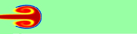
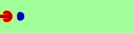
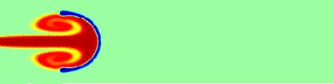
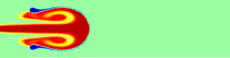
The figures show the jet pushing the bubble for times t=1, 4, 6, 8.

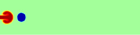
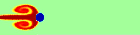
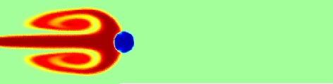
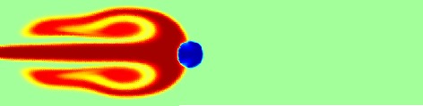
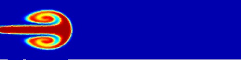
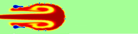
Breaking bubbles

What happens if we lower the surface tension? Set now

GfsSourceTension T1 0.01 K

The figures show the jet pushing the bubble which now ... breaks!! (for times t=1, 4, 6, 8).

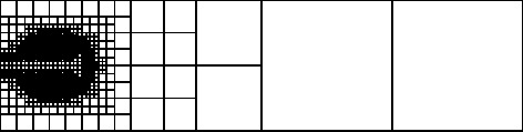
and the grid and a little (big) zoom for time t=8

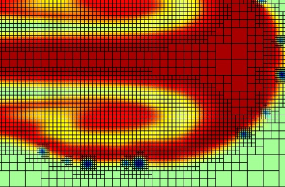
It is interesting to note that in the grid figure above Gerris uses 3232 mesh points (or squares). Without adaptive mesh refinement we must set 4 boxes of 64x64 or more of 128x128 because the frontier needs a 7 level refinement so 3232 or 16384 or 65538, you have the choice.

Gerris in parallel

One of man's dreams is to run a program in parallel. Gerris allows to do this quite easily, for instance if you want run our last script on four processors we have to modify only the boundary conditions using the Gerris keyword pid like

4 3 GfsSimulation GfsBox GfsGEdge {} {
  Refine 5
  Time { end = 20 }
  VariableTracer T
  VariableTracerVOF T1
  InitFraction T1 ((x)*(x) + y*y - 0.125*0.125)
  VariableCurvature K T1
  SourceTension T1 0.01 K
  SourceViscosity 1./400
  AdaptGradient { istep = 1 } { maxlevel = 7 cmax = 1e-2 } T1
  AdaptGradient { istep = 1 } {maxlevel = 6 cmax = 1e-2} T
  OutputTime { step = 1 } stderr
  OutputSimulation { step = 1 } stdout
}
GfsBox {
  pid = 0
  top  =  Boundary {
    BcDirichlet U 0
    BcDirichlet V 0
  }
  bottom  =  Boundary {
    BcDirichlet U 0
    BcDirichlet V 0
  }
  left = Boundary {
    BcDirichlet U ( (y > -0.05 && y < 0.05 ) ? 1 : 0 )	   
    BcDirichlet T ( (y > -0.05 && y < 0.05 ) ? 1 : 0 )
  }
}
GfsBox { pid = 1 }
GfsBox { pid = 2 }
GfsBox {
    pid = 3
    right = BoundaryOutflow
}
1 2 right
2 3 right
3 4 right

and run the script with

mpirun -np 4 gerris2D tutorial2.gfs

What we do is an example of manually partitioning the domain. In more complex cases, Gerris can also automatically partition the domain for a given number of processors, variable resolution, complex boundaries.

Therefore we can now begin a good Saturday night saying

You know sweet, I can run parallel programs...

success assured!!