6.1 PASS:
Lid-driven cavity at Re=1000
-
Author
- Stéphane Popinet
- Command
- sh lid.sh lid.gfs
- Version
- 0.6.4
- Required files
- lid.gfs (view) (download)
lid.sh xprofile yprofile xprof.ghia yprof.ghia
- Running time
- 3 minutes 39 seconds
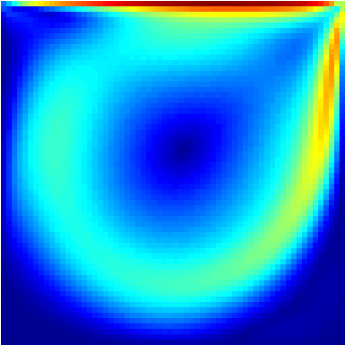
The classical lid-driven cavity test case.
This example illustrates how to check for the convergence toward a
stationary solution of an initially time-dependent problem.
The stationary solution obtained is illustrated on Figure 78.
| Figure 78: Norm of the velocity for the stationary regime. |
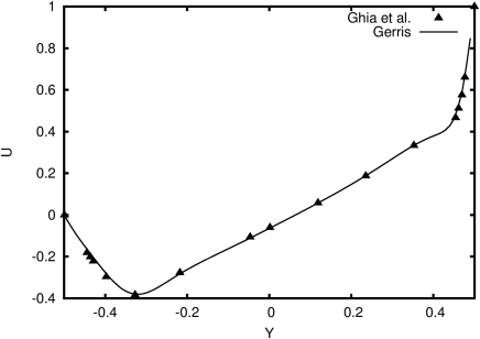
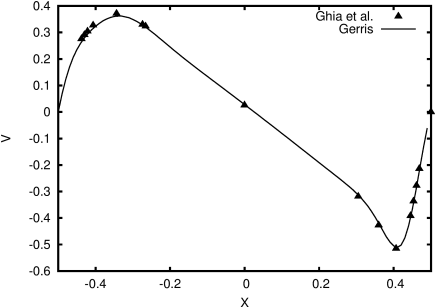
Velocity profiles are generated automatically and compared to the
benchmark results of Ghia et al. [44] on
Figures 79 and 80.
| Figure 79: Vertical profile of the x-component of the velocity on
the centerline of the box. |
| Figure 80: Horizontal profile of the y-component of the velocity on
the centerline of the box. |
6.1.1 PASS:
Lid-driven cavity at Re=1000 (explicit scheme)
-
Author
- Stéphane Popinet
- Command
- sh lid.sh explicit.gfs
- Version
- 1.3.0
- Required files
- explicit.gfs (view) (download)
lid.sh
- Running time
- 2 minutes 37 seconds
Same test case but with an explicit scheme for the viscous term.
6.1.2 PASS:
Lid-driven cavity on an anisotropic mesh
-
Author
- Sébastien Delaux
- Command
- sh ../lid.sh stretch.gfs
- Version
- 100208
- Required files
- stretch.gfs (view) (download)
xprofile yprofile xprof.ghia yprof.ghia
- Running time
- 16 minutes 58 seconds
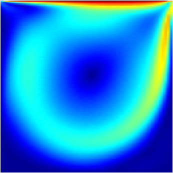
Same test case except that the domain is made of two boxes instead
of one. The stretch metric is used to transform the rectangular
domain into a square one.
The stationary solution obtained is illustrated on Figure 81.
| Figure 81: Norm of the velocity for the stationary regime. |
Velocity profiles are generated automatically and compared to the
benchmark results of Ghia et al. [44] on
Figures 82 and 83.
| Figure 82: Vertical profile of the x-component of the velocity on
the centerline of the box. |
| Figure 83: Horizontal profile of the y-component of the velocity on
the centerline of the box. |
6.1.3 PASS:
Lid-driven cavity with a non-uniform metric
-
Author
- Stéphane Popinet
- Command
- sh ../lid.sh metric.gfs
- Version
- 111025
- Required files
- metric.gfs (view) (download)
isolines.gfv xprofile yprofile xprof.ghia yprof.ghia
- Running time
- 22 minutes 10 seconds
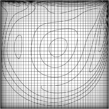
Same test case but using a non-uniformly-stretched mesh in both
directions.
The stationary solution obtained is illustrated on Figure
84 together with the non-uniform mesh.
| Figure 84: Isolines of the norm of the velocity for
the stationary regime and non-uniform mesh. |
Velocity profiles are generated automatically and compared to the
benchmark results of Ghia et al. [44] on
Figures 85 and 86.
| Figure 85: Vertical profile of the x-component of the velocity on
the centerline of the box. |
| Figure 86: Horizontal profile of the y-component of the velocity on
the centerline of the box. |