The spherical harmonics are by definition a family of functions which satisfy the Laplace equation on the sphere
| ∇2 f = |
|
| ⎛ ⎜ ⎜ ⎝ | r2 |
| ⎞ ⎟ ⎟ ⎠ | + |
|
| ⎛ ⎜ ⎜ ⎝ | sinθ |
| ⎞ ⎟ ⎟ ⎠ | + |
|
| = 0. |
If we look for solutions of the form f (r, θ, ϕ) = R (r) Y (θ, ϕ), then two differential equations result. If we consider only the equation for the angles, we get
|
|
| ⎛ ⎜ ⎜ ⎝ | sinθ |
| ⎞ ⎟ ⎟ ⎠ | + |
|
|
| = − λ |
were λ is a constant. This equation has a whole range of solutions noted Ylm (θ, ϕ) so that
| ∇ Ylm (θ, ϕ) = − l (l + 1) Ylm (θ, ϕ) . |
The Ylm can be expressed as functions of the Legendre polynomials as
| Ylm (θ, ϕ) = |
|
| Plm (cosθ) cos(m ϕ) |
where Plm is the associated Legendre polynomial.
For this test we used l = 4 and m = 2.
Figure 165: Solution to the Poisson problem with a pure spherical harmonic solution, as represented on the "developed cubed sphere". 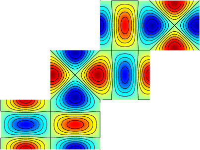
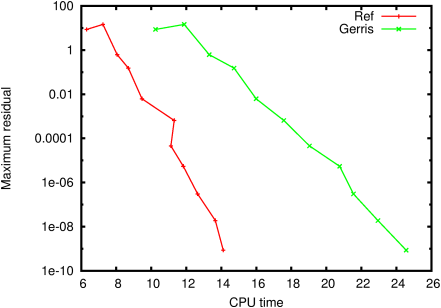
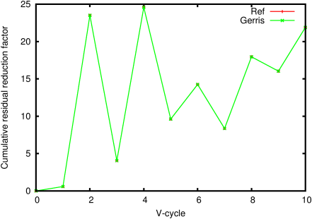
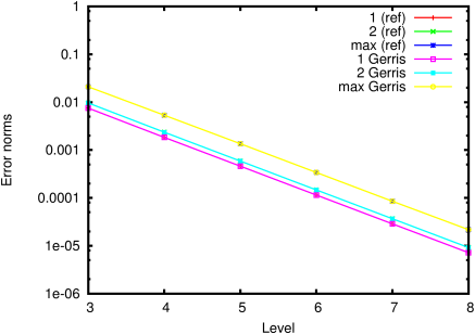
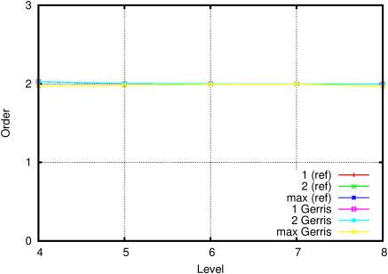
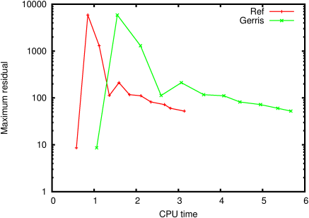
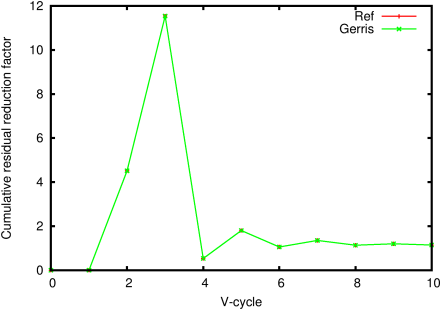
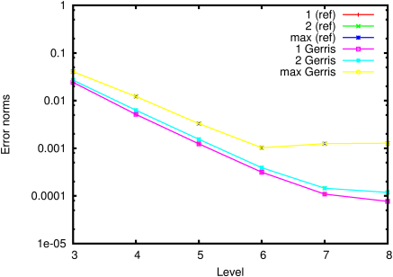
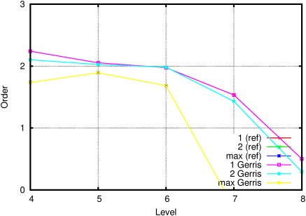
Figure 166 illustrates the evolution of the maximum residual as a function of CPU time. Figure 167 illustrates the average residual reduction factor (per V-cycle). The evolution of the norms of the error of the final solution as a function of resolution is illustrated on Figure 168. The corresponding order of convergence is given on Figure 169.
Same test case but using longitude-latitude spherical coordinates.
Figure 170: Solution to the Poisson problem with a pure spherical harmonic solution, as represented on the longitude-latitude coordinate system. 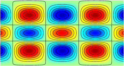
Figure 171 illustrates the evolution of the maximum residual as a function of CPU time. Figure 172 illustrates the average residual reduction factor (per V-cycle). The evolution of the norms of the error of the final solution as a function of resolution is illustrated on Figure 173. The corresponding order of convergence is given on Figure 174.
While initial convergence is satisfactory, the pole singularities quickly dominate the error. The convergence rate of the multigrid solver is also low, due to the large scale ratio induced by the metric. Better solutions at high-resolution can be obtained by increasing the number of iterations of the multigrid solver, but at a large computational cost.