13.2 PASS:
Advection of a cosine bell around the sphere
-
Author
- Stéphane Popinet
- Command
- sh cosine.sh
- Version
- 091029
- Required files
- cosine.gfs (view) (download)
cosine.sh isolines.gfv reference.gfv zero.gfv error-45.ref error-90.ref rossmanith45 rossmanith90
- Running time
- 2 minutes 44 seconds
This test case was suggested by Williamson et
al. [47] (Problem #1). A "cosine bell" initial
concentration is given by
| h(λ,θ)=(h0/2)(1+cos(π r/R))
|
if r<R and 0 otherwise, with R=1/3 and
| r=arccos[sinθcsinθ+cosθccosθcos(λ−λc)]
|
the great circle distance between longitude, latitude
(λ,θ) and the center initially taken as
(λc,θc)=(3π/2,0).
The advection velocity field corresponds to solid-body rotation at an
angle α to the polar axis of the spherical coordinate
system. It is given by the streamfunction
| ψ=−u0(sinθcosα−cosλcosθsinα)
|
The cosine bell field is rotated once around the sphere and should
come back exactly to its original position. The difference between
the initial and final fields is a measure of the accuracy of the
advection scheme coupled with the spherical coordinate mapping (the
"conformal expanded spherical cube" metric in our case).
For the "spherical cube" metric, two angles are considered: 45
degrees which rotates the cosine bell above four of the eight "poles"
of the mapping and 90 degrees which avoids the poles entirely. Mass
is conserved to within machine accuracy in either case.
The mesh is adapted dynamically according to the gradient of tracer
concentration.
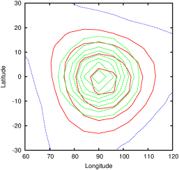
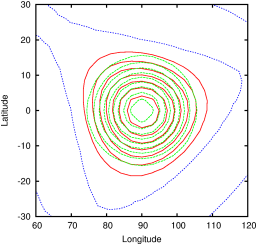
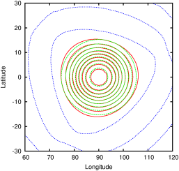
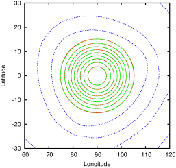
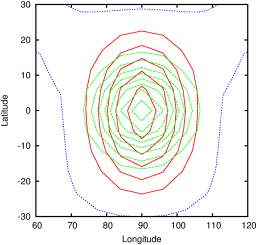
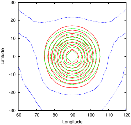
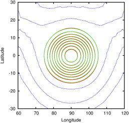
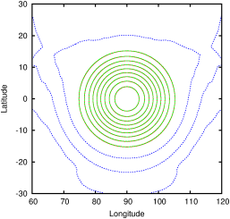
| Figure 161: Tracer field after one rotation around the
sphere with α=45∘ (red). Reference solution
(green). Zero level contour line (blue). Equivalent static
resolutions (a) 16× 16× 6. (b) 32× 32×
6. (c) 64× 64× 6. (d) 128× 128× 6. |
| Figure 162: Tracer field after one rotation around the
sphere with α=90∘ (red). Reference solution
(green). Zero level contour line (blue). Equivalent static
resolutions (a) 16× 16× 6. (b) 32× 32×
6. (c) 64× 64× 6. (d) 128× 128× 6. |
| Figure 163: Relative error norms (as defined in
[47]) as functions of spatial resolution. The results
of Rossmanith [38] using a gnomonic spherical cube
metric and a different 2nd-order advection scheme are also
reproduced for comparison. (a) α=45∘. (b)
α=90∘. |
(a) 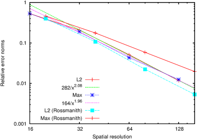 |
(b) 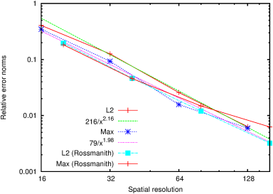 |
| Figure 164: Maximum relative errors as functions of
time. (a) α=45∘. (b) α=90∘. |
(a) 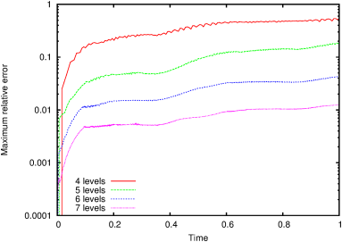 |
(b) 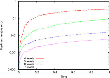 |