11.1 PASS:
Geostrophic adjustment
-
Author
- Stéphane Popinet
- Command
- sh geo.sh geo.gfs
- Version
- 100323
- Required files
- geo.gfs (view) (download)
geo.sh geo.gfv e.ref
- Running time
- 2 minutes 46 seconds
We consider the geostrophic adjustment problem studied by
Dupont [14] and Le Roux et al [24]. A Gaussian bump
is initialised in a 1000×1000 km, 1000 m deep square basin. A reduced
gravity g = 0.01 m/s2 is used to approximate a 10 m-thick stratified surface
layer. On an f-plane the corresponding geostrophic velocities are given by
where f0 is the Coriolis parameter. Following Dupont we set f0 = 1.0285
× 10− 4 s− 1, R = 100 km, η0 = 599.5 m which gives a
maximum geostrophic velocity of 0.5 m/s.
In the context of the linearised shallow-water equations, the geostrophic
balance is an exact solution which should be preserved by the numerical
method. In practice, this would require an exact numerical balance between
terms computed very differently: the pressure gradient and the Coriolis terms
in the momentum equation. If this numerical balance is not exact, the
numerical solution will adjust toward numerical equilibrium through the
emission of gravity-wave noise which should not affect the stability of the
solution. This problem is thus a good test of both the overall accuracy of the
numerical scheme and its stability properties when dealing with
inertia–gravity waves. We note in particular that a standard A-grid
discretisation would develop a strong computational-mode instability in this
case. Also, as studied by Leroux et al, an inappropriate choice of
finite-element basis functions will result in growing gravity-wave noise.
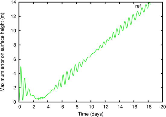
| Figure 128: Evolution of the maximum error on the surface height for the
geostrophic adjustment problem. |
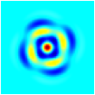
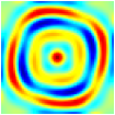
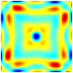
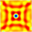
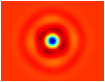
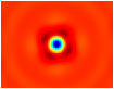
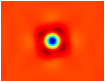
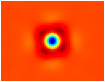
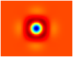
| Figure 129: Evolution of the surface-height error field. (a) t =1.157
days, (b) t = 2.315 days, (c) t =3.472 days, (d) t =4.630 days, (e) t
=17.361 days. |
Figures 128 and 129 summarise the results obtained
when running the geostrophic adjustment problem on a 64 × 64 uniform
grid with a timestep Δ t = 1000 s. The maximum error on the height
field (Figure 128) is small even after 18 days. After a strong
initial transient corresponding to the emission of gravity waves, the error
reaches a minimum at day 3 and then slowly grows with time with modulations
due to the reflexions of the initial gravity waves on the domain boundaries.
As illustrated on figure 129, this growth is not due to any
instability of the solution but to the slow decrease of the maximum amplitude
of the Gaussian bump due to numerical energy dissipation.
11.1.1 PASS:
Geostrophic adjustment on a beta-plane
-
Author
- Stéphane Popinet
- Command
- sh beta.sh beta.gfs
- Version
- 100323
- Required files
- beta.gfs (view) (download)
beta.sh c dlw lls pzm llw energy.ref energy-nonlinear.ref
- Running time
- 6 minutes 42 seconds
Same as before but a beta-plane, f = f0 + β y is used and
the advection terms are included in the momentum equation. No
explicit dissipation is added. As in [14] we chose β
= 1.607 × 10− 11 m− 1s− 1. The geostrophic eddy
moves slowly westward through the emission of Rossby waves and
southward due to the non-linear advection term. The resulting
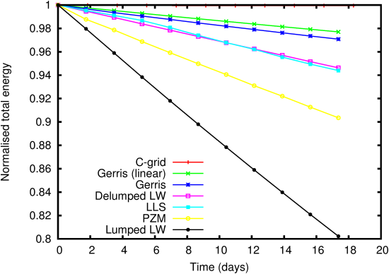
evolution of the total energy is shown on figure 130. For
our method, the slow decrease in the total energy is due both to the
dissipation of potential energy induced by the approximate
projection operator and to the dissipative properties of the BCG
upwind advection scheme. Another run with the advection terms
switched off (figure 130, green curve) confirms that the
dissipation induced by the approximate projection operator dominates
the total dissipation. The results however compare favourably with
the finite-element formulations tested by Dupont which all show
significantly larger energy dissipation.
| Figure 130: Evolution
of the total energy for the non-linear geostrophic adjustment problem. The
C-grid model is based on Sadourny [] and implemented by Dupont
[14]. The finite-element formulations are those studied by Dupont. LW:
Lynch and Werner [27], LLS: Le Roux et al [24], PZM: Peraire et al
[30]. |
11.1.2 PASS:
Geostrophic adjustment with Saint-Venant
-
Author
- Stéphane Popinet
- Command
- sh geo.sh river.gfs
- Version
- 130112
- Required files
- river.gfs (view) (download)
geo.sh geo.gfv e.ref
- Running time
- 42 seconds
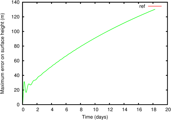
Same test but using the (fully nonlinear) Saint-Venant solver.
| Figure 131: Evolution of the maximum error on the surface height for the
geostrophic adjustment problem. |
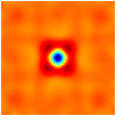
| Figure 132: Evolution of the surface-height error field. (a) t =1.157
days, (b) t = 2.315 days, (c) t =3.472 days, (d) t =4.630 days, (e) t
=17.361 days. |