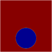
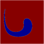
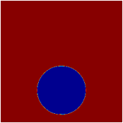
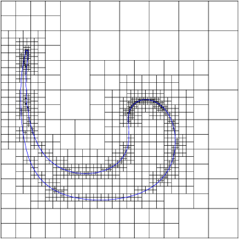
A test case initially presented by Rudman [39]. A circular patch of tracer is advected in a vortical shear flow. At t = 2.5 the flow direction is reversed. An exact advection scheme would restore the initial circular shape at t = 5.
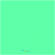
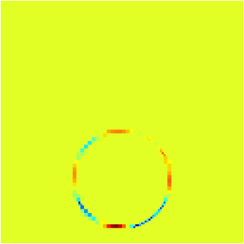
The VOF (Volume-Of-Fluid) advection scheme is not exact. The initial, intermediate and final shape of the interface are represented on Figure 35. Figure 36 illustrates the error between the initial and final shapes. The corresponding error norms are given in Table 1.
Adaptive refinement is used with the gradient of the volume fraction as criterion. Eight levels of refinement are used on the interfaces and six away from the interface.
(a) (b) (c)
Table 1: Norms of the error between the initial and final fields. The reference values are given in blue.
L1 L2 L∞ 1.665e-04 5.445e-03 3.622e-01 1.672e-04 5.458e-03 3.626e-01
Same as the previous test but with adaptivity based on the local curvature of the interface (with a maximum of eight levels of refinement).
Table 2: Norms of the error between the initial and final fields. The reference values are given in blue.
L1 L2 L∞ 8.775e-04 8.309e-03 1.965e-01 8.775e-04 8.309e-03 1.965e-01
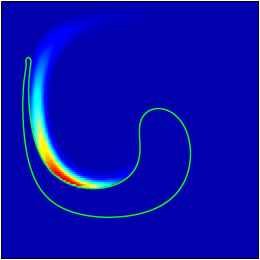
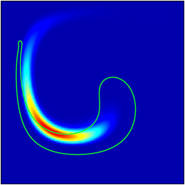
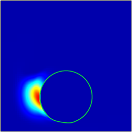
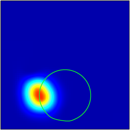
A similar test but with the addition of a concentration field (C) associated with the VOF tracer (i.e. the phase with T > 0). The initial concentration field is a Gaussian bump. The maximum of the bump is located on the VOF interface to emphasise errors in the advection of the VOF concentration. For reference a standard (Godunov) tracer (G) is added, initialised with the same initial Gaussian bump. Ideally C should match G when T > 0 and both C and G should return to the initial Gaussian distribution at t=5.
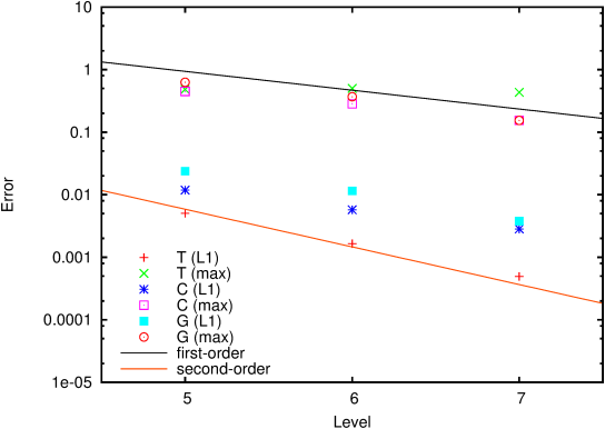
The VOF interface and tracer fields are illustrated in Figure 39. The corresponding convergence of the error norms with spatial resolution is illustrated in Figure 40.
The VOF tracer is conserved to within 10−4, C to within 2× 10⁻⁵ (at the coarsest resolution) and G exactly.