6.7 PASS:
Wind-driven lake
-
Author
- Stéphane Popinet
- Command
- gerris2D lake.gfs
- Version
- 110325
- Required files
- lake.gfs (view) (download)
lake.gfv
- Running time
- 1 minutes 18 seconds
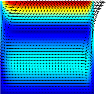
A simple test of a wind-driven lake with a 1/10 mesh stretching
ratio. Due to the anisotropy of stretching, the hypre module needs
to be used to solve the Poisson and diffusion problems
efficiently. Further, with Neumann boundary conditions everywhere
for the pressure, the resulting linear system is rank-deficient and
needs to be "fixed" to avoid drift problems in HYPRE.
| Figure 94: Norm of the velocity and vectors for the
stationary regime. The vertical scale is stretched by a factor of
ten. |
6.7.1 PASS:
Multi-layer Saint-Venant solver
-
Author
- Stéphane Popinet
- Command
- sh river.sh
- Version
- 120717
- Required files
- river.gfs (view) (download)
river.sh error.ref
- Running time
- 21 seconds
A similar test but using the multi-layer hydrostatic Saint-Venant
solver.
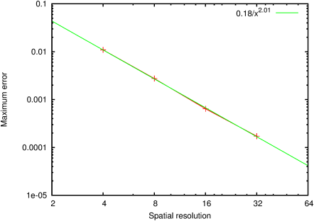
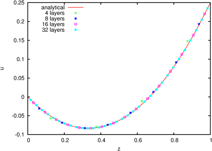
Figure 95 illustrates the velocity profile at the center of
the lake and Figure 96 the rate of convergence with an
increasing number of layers.
| Figure 95: Numerical and analytical velocity profiles at
the center of the lake. |
| Figure 96: Convergence of the error between the numerical
and analytical solution with the number of layers. |
6.7.2 PASS:
Wind-driven stratified lake
-
Author
- Stéphane Popinet
- Command
- sh stratified.sh
- Version
- 121116
- Required files
- stratified.gfs (view) (download)
stratified.sh error.ref field.awk thermo.awk
- Running time
- 1 minutes 46 seconds
We now consider the case of a stratified lake. To model the stable
thermal stratification often observed in lakes, we assume a vertical
density profile of the form
| ρ (z) = ρ0 − Heaviside (z − H +
Hthermocline) Δ ρ . |
If Δ ρ / ρ0 is small compared to one, we can use a
Boussinesq approximation and this results in an additional source
term − g′ Heaviside (z − H + Hthermocline) for
the vertical component of velocity, with g′ the reduced gravity
Through dimensional arguments one can find that the equilibrium
slope αt of the thermocline should verify the relation
for vanishing αt.
We then need to consider two additional independent dimensionless
parameters
-
b = 1 − Hthermocline / H, set to 3 / 4 in what follows,
- and the thermocline slope
If we assume parallel flow, an analytical solution can be sought for
the horizontal velocity profile in a vertical cross-section, of the
form
| u (z) = A1 z2 + B1 z + C1 | | for z > b, |
| u (z) = A2 z2 + B2 z + C2 | | for z ≤ b |
|
Using boundary and volume conservation conditions one easily finds
(for b = 3 / 4)
| | for z > 3 / 4, |
| | for z ≤ 3 / 4. |
|
This can be used to refine the estimates of the thermocline and surface
slopes. Assuming hydrostatic balance, the horizontal pressure gradient is
given by
| ∂x p = g α′ | | for z > 3 / 4 + αt′ x, |
| ∂x p = g α′ + g′ αt′ | | for z ≤ 3 / 4 +
αt′ x. |
|
Balancing the horizontal pressure gradients and viscous stress then gives
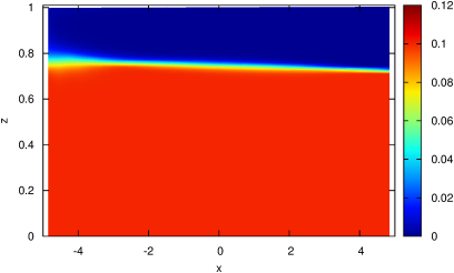
The (pseudo) steady-state density perturbation is illustrated in
Figure 97 and the corresponding free-surface and thermocline
slopes in Figure 100.
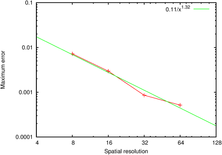
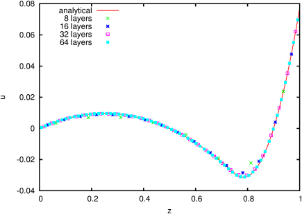
Figure 98 illustrates the velocity profile at the center of the
lake and Figure 99 the rate of convergence with an
increasing number of layers.
| Figure 97: Density perturbation Δρ for 64
layers. Numerical diffusion is most noticeable in the upwelling on
the left-hand-side. |
| Figure 98: Numerical and analytical velocity profiles at
the center of the lake. |
| Figure 99: Convergence of the error between the numerical
and analytical solution with the number of layers. |
| Figure 100: Profiles of (a) the free surface and (b)
the thermocline compared with the analytical solutions. |
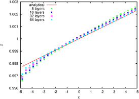 | 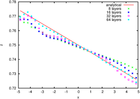 |
| (a) | (b) |