This test case is taken from the test cases of the Advanced Regional Prediction System [13]. A Coriolis term is applied to a cubic domain with periodic boundary conditions in the x, y and z directions. Provided the flow has a unidirectional initial velocity field and a zero initial pressure perturbation, the spatial derivatives are initially zero and a solution exists to the Navier-Stokes equations for which spatial derivatives are zero at all times.
In this case the velocity field is given by:
| u = A cos(2Ω t) + B sin(2Ω t) |
| v = − A sinΦ sin(2Ω t) + B sinΦ cos(2Ω t) + C |
| w = A cosΦ sin(2Ω t) − B cosΦ cos(2Ω t) + D |
where A, B, C and D are constants of integration:
| A = U0 |
| B = sinΦ V0 − cosΦ W0 |
| C = cosΦ | ⎛ ⎝ | cosΦ V0 + sinΦ W0 | ⎞ ⎠ |
| D = sinΦ | ⎛ ⎝ | cosΦ V0 + sinΦ W0 | ⎞ ⎠ |
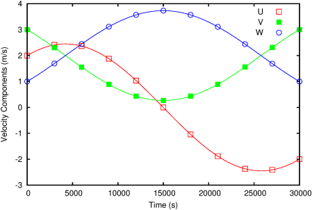
Here Φ = π/2 so that the z component of the Coriolis force is equal to zero. Figure 93 shows the evolution of the three components of the velocity with time.