The simplest model of groundwater flow is provided by Darcy’s law [6]: construed on the macroscopic scale, at which individual pores are invisible, the ‘discharge’ velocity u is divergence-free
| ∇·u = 0 |
and proportional to the hydraulic gradient ∇ p:
| u = − k∇ p . |
The coefficient of proportionality k is known as the permeability or hydraulic conductivity, and may in general vary from place to place or be a second-order tensor; for this first test it is taken as constant.
Such a problem can be solved by Gerris using its projection method: one turns off the advection and does not activate viscosity. Darcy’s law itself is provided by linear implicit GfsSourceCoriolis terms. The standard GfsSimulation solver then works as a false-transient iteration toward the steady-state, which will be correct if the pressure converges, implying a divergence-free discharge velocity.
The following example is based on Figure 5-3 of Harr [19][p. 146], but converted from rectangular to circular geometry so as to permit a simple closed-form solution: a uniform aquifer confined to an annular sector, with impermeable arcs and different constant heads imposed on the two radii. The exact solution has the head constant along radii and varying linearly with angle.
Figure 212: Isobars and velocity vectors for Darcy flow in a confined annular sector aquifer with separate reservoir and drain. 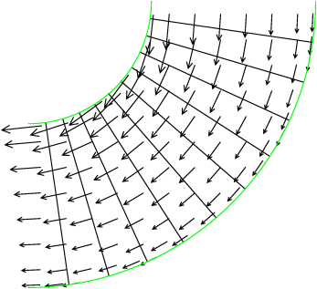
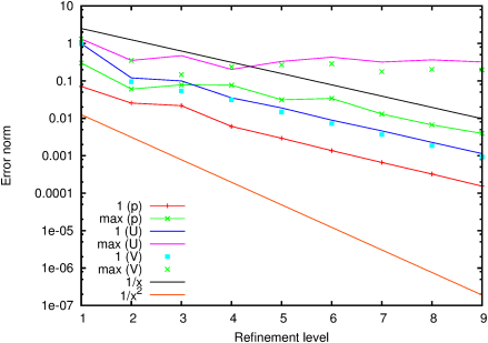
Figure 213: Grid-convergence of the pressure and velocity, for Darcy flow in a confined annular sector aquifer with separate reservoir and drain. 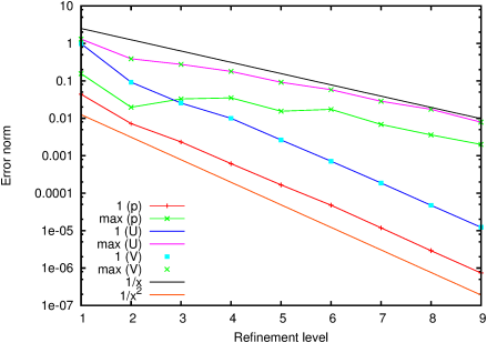
Discontinuities of hydraulic conductivity are common in groundwater flow. They can be handled by Gerris’s projection method using the alpha keyword in GfsPhysicalParams.
Even with nonuniform porosity, the discharge velocity will be divergence-free [6, p. 198] (assuming only that the local liquid density is constant). Applying that condition to Darcy’s flux law yields
| ∇· | ⎛ ⎝ | k∇ p | ⎞ ⎠ | = ∇·u , |
which closely resembles the projection Poisson equation used in Gerris [32, eq. 7]:
| ∇· | ⎡ ⎢ ⎢ ⎢ ⎢ ⎣ |
| ∇ p |
| ⎤ ⎥ ⎥ ⎥ ⎥ ⎦ | = ∇·u*. |
noting that the (here false) time-step Δ t will be uniform in space and so can be taken outside the divergence, all that is required is to identify the ‘density’ ρn+1/2 with something inversely proportional to the permeability. As Gerris is told about this density via its reciprocal alpha in GfsPhysicalParams, we just that proportional to permeability.
In many soils, the permeability varies in proportion to the porosity [19, p. 94], so this alpha factor can be seen as the porosity too, in which case it reflects the difference between the ‘discharge’ and ‘seepage’ velocities, the first being the one that is calculated by Gerris and corresponding to macroscopic measurements while the latter is that in the pores. The relation between the two is simply that the discharge velocity is the seepage velocity times the porosity [6, p. 23].
Here we modify the first example by halving the porosity in the last third of the aquifer (so that it has the same total hydraulic resistance as the first two thirds). The exact solution has the velocity field exactly as before, but with a steeper azimuthal pressure gradient beyond porosity jump at θ < −π/3.
Figure 214: Isobars and velocity vectors, for Darcy flow in a confined annular sector aquifer with separate reservoir and drain, and halved permeability in the most-clockwise third sector. 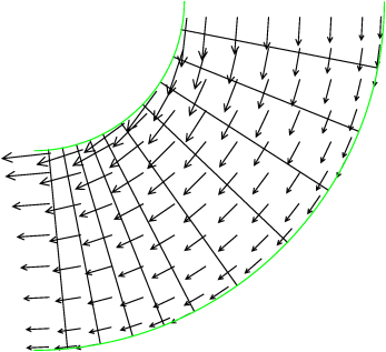
Figure 215: Grid-convergence of the pressure and velocity, for Darcy flow with piecewise constant permeability.