This example is a classical validation test case for tsunami models. It was proposed at the "Third international workshop on long-wave runup models". It is based on experimental data obtained in a wave tank in order to understand the extreme runups observed near the village of Monai during the 1993 Okushiri tsunami.
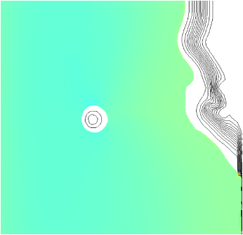
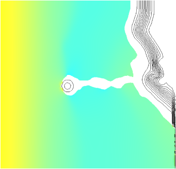
The animation in Figure 42 gives a general idea of the geometry and time evolution of the modelled tsunami. The bathymetry data and channel geometry matches that used in the experimental wave tank. The water surface is forced on the open boundary with the experimentally-imposed waveform (outside the field of view on the right-hand-side in the animation). The initial dryout as well as extreme runup in the narrow central valley are clearly visible in the animation, as well as wave reflections from the boundaries and dimples in the water surface caused by underwater vortices.
Figure 42: Animation of the water surface (light blue) and bathymetry (white) for the Monai tsunami. 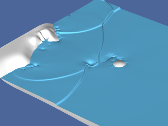
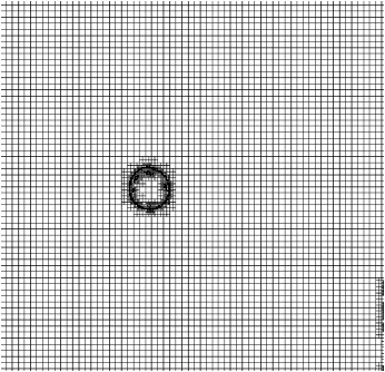
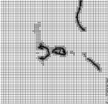
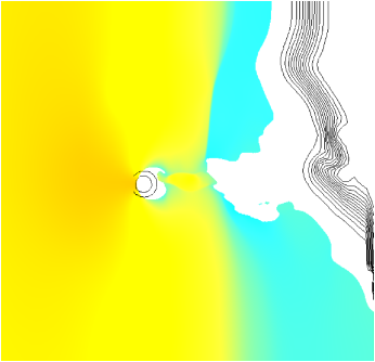
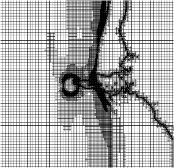
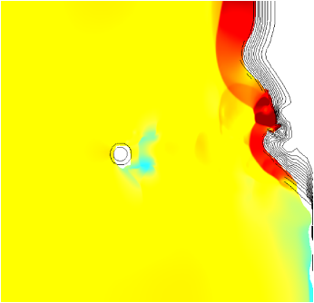
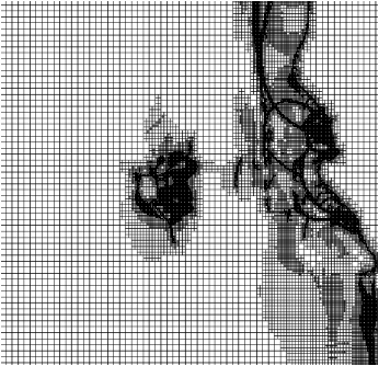
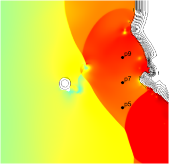
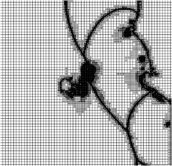
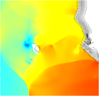
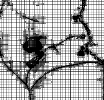
Another view of the process together with the adaptive mesh used to resolve the flow is given in Figure 43. This figure can be compared with that of LeVeque and George (Figure 4 of [7]).
t = 10 s t = 12 s t = 14 s t = 16 s t = 18 s t = 20 s
Experimental data includes free-surface elevation timeseries at several locations (see Figure 43, t = 18 s). Figures 44, 45 and 46 give comparisons of the experimental and numerical timeseries.
Figure 44: Time-series of free-surface elevation measured and calculated at the location of probe 5. 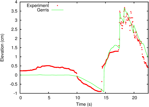
Figure 45: Time-series of free-surface elevation measured and calculated at the location of probe 7. 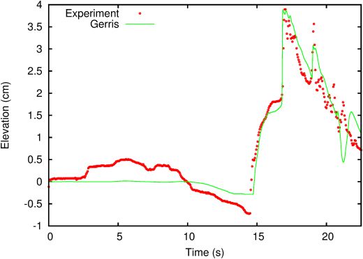
Figure 46: Time-series of free-surface elevation measured and calculated at the location of probe 9. 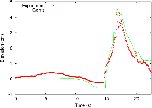
Finally, the animation in Figure 47 gives a comparison between the overhead video of the experiment and the corresponding view of the simulation.
Figure 47: Comparison between the video of the experiment (left) and the simulation results (right). 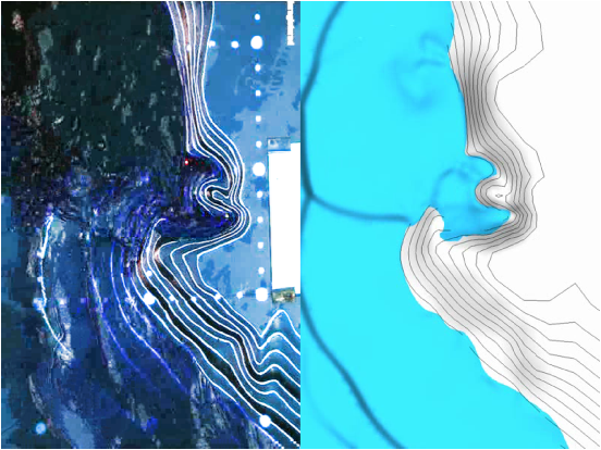
More details on this simulation and the method used is given in [9].