3.5 Forced isotropic turbulence in a triply-periodic box
-
Author
- Kristjan Gudmundsson
- Command
- mpirun -np 8 gerris3D -m -s1 forcedturbulence.gfs
- Version
- 110131
- Required files
- forcedturbulence.gfs (view) (download)
spectral.dat multiview.gfv
- Running time
- 22 hours on 8 AMD Opteron 2GHz
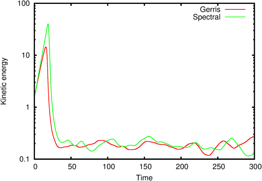
We compute the evolution of forced isotropic turbulence (see
[10]) and compare Gerris’ solution to that of the
hit3d
pseudo-spectral code. The initial condition is an unstable solution
to the incompressible Euler equations. Numerical noise in the
solution eventually leads to the destabilisation of the base
solution into a fully turbulent flow where turbulent dissipation
balances the linear input of energy (as illustrated graphically in
the animation of Figure 26).
The two codes agree at early time, or until the solution transitions
to a turbulent state. This happens earlier in Gerris as the symmetry
of the base state is not preserved with the same accuracy as in the
pseudo-spectral code (the main reason being the tolerance on
non-divergence of the incompressible velocity field). Note however
that the statistics produced by the two codes agree well after
transition to turbulence.
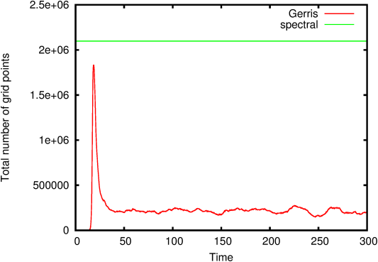
Adaptivity is used in Gerris to reduce the computational
cost. Figure 30 illustrates the number of grid points as a
function of time.
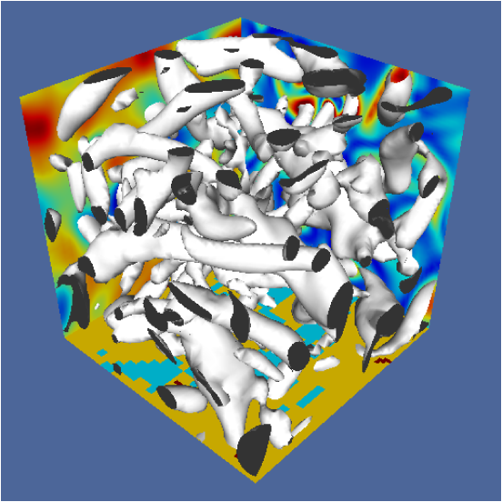
| Figure 26: Animation of the evolution of the
λ2 isosurface (a way to characterise vortices),
cross-sections of the level of refinement (bottom plane), of the
magnitude of vorticity (right plane) and pressure (left plane). |
| Figure 27: Evolution of kinetic energy as computed via
Gerris and a pseudo-spectral code. Note how the energy grows
exponentially before the flow finally transitions to
turbulence. This is because the laminar solution is relatively
smooth and its dissipation is unable to balance the energy input. |
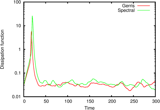
| Figure 28: The dissipation function. The
dissipation increases exponentially during the laminar stage as it
is proportional to energy at this stage. During transition the
dissipation increases drastically as the flow gains energy at higher
wavenumbers. |
| Figure 29: The microscale Reynolds number. |
| Figure 30: Number of grid points as a function of time for
Gerris and the spectral code. |