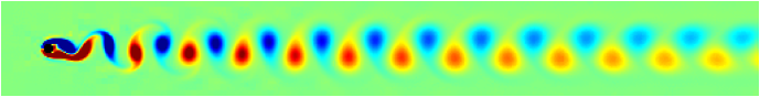
An example of 2D viscous flow around a simple solid boundary. Fluid is injected to the left of a channel bounded by solid walls with a slip boundary condition. A passive tracer is injected in the bottom half of the inlet.
Adaptive refinement is used based on both the vorticity and the gradient of the passive tracer.
After an initial growth phase, a classical Bénard–von Kárman vortex street is formed.
The results are visualised using MPEG movies of the vorticity (Figure 1) and tracer concentration (Figure 2) generated on-the-fly.
Same as the previous example but this time the tracer is "passive temperature" (i.e. the change in density due to heating is assumed to be negligible).
This is an example on how to solve an advection–diffusion equation for a tracer with Dirichlet boundary conditions on an immersed solid boundary.
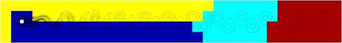
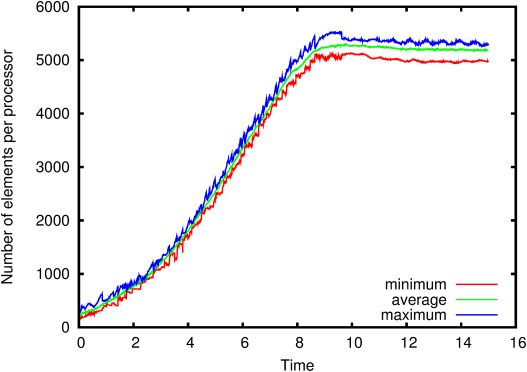
The simulation is run in parallel on four processors. Load balancing is used to dynamically redistribute the elements across processors in order to maintain roughly equal mesh sizes on each processor as the resolution varies due to adaptive mesh refinement.
Figure 4: MPEG movie of the processor number assigned to each cell (colour field) together with isolines of vorticity.