4.1 PASS:
Estimation of the numerical viscosity
-
Author
- Stéphane Popinet
- Command
- sh reynolds.sh reynolds.gfs 1
- Version
- 0.6.4
- Required files
- reynolds.gfs (view) (download)
reynolds.sh div5.ref div6.ref div7.ref reynolds.ref
- Running time
- 3 minutes 26 seconds
The velocity field is initialised with an exact stationary solution of
the Euler equations in a periodic 2D domain. An exact Euler solver
would not change this field, however any numerical solver will
introduce numerical dissipation which will slowly dissipate the
kinetic energy of the initial solution. By monitoring the evolution of
the kinetic energy, the dissipative properties of the numerical scheme
can be measured (see [37] for details).
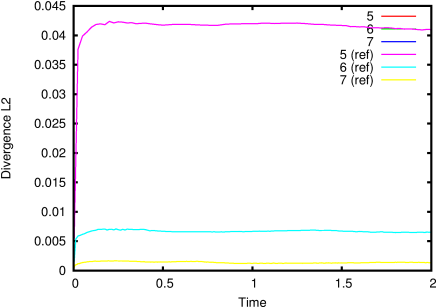
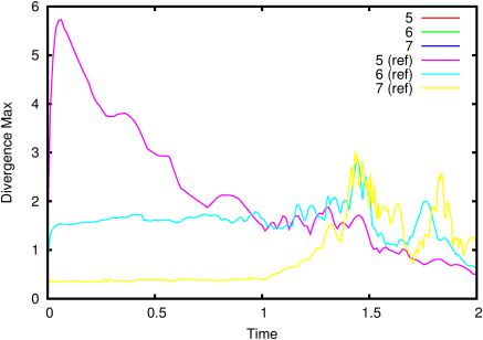
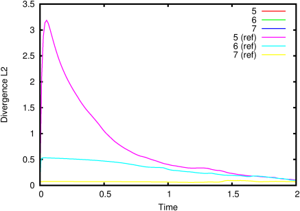
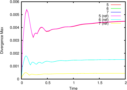
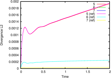
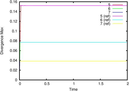
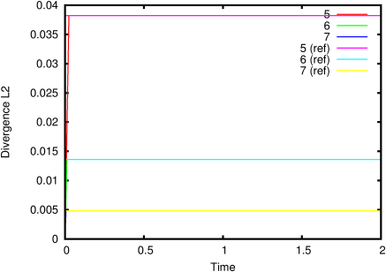
Figures 45 and figure 46 illustrate the evolution
of the divergence of the velocity field with time. This is a check of
the stability of the approximate projection and should remain bounded.
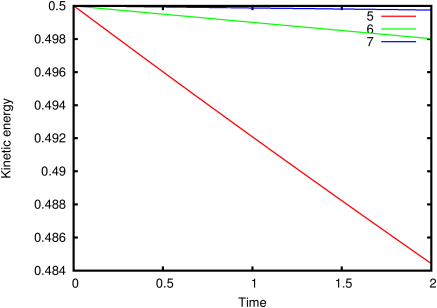
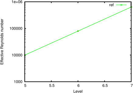
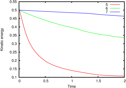
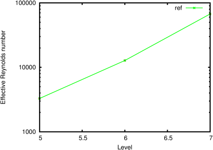
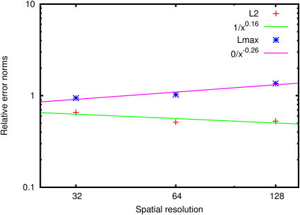
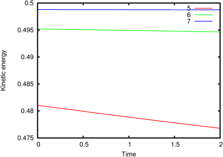
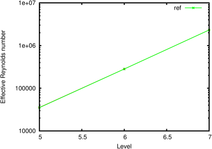
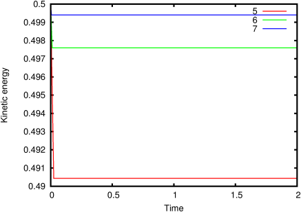
Figures 47 and 48 illustrates the evolution of
the kinetic energy and the corresponding equivalent Reynolds number as
a function of resolution. The higher the Reynolds number, the less
dissipative the scheme.
| Figure 45: Evolution of the maximum divergence. |
| Figure 46: Evolution of the L2 norm of the divergence. |
| Figure 47: Evolution of the kinetic energy. |
| Figure 48: Equivalent Reynolds number as a function of resolution. |
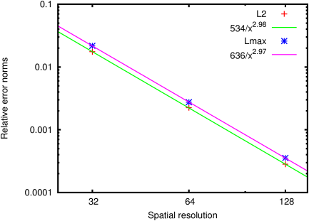
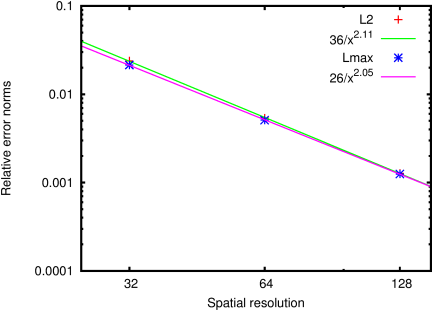
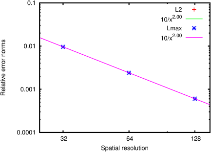
| Figure 49: Accuracy of the solution as a function of the level of refinement. |
4.1.1 PASS:
Estimation of the numerical viscosity with refined box
-
Author
- Stéphane Popinet
- Command
- sh ../reynolds.sh box.gfs 4
- Version
- 0.6.4
- Required files
- box.gfs (view) (download)
../reynolds.sh div5.ref div6.ref div7.ref reynolds.ref
- Running time
- 19 minutes 45 seconds
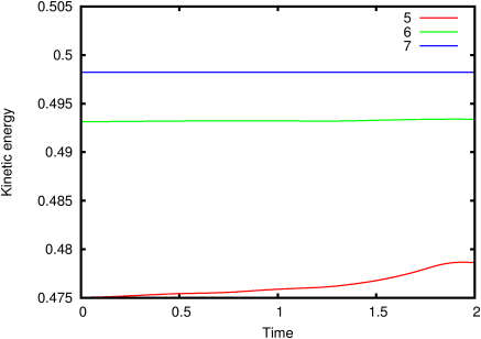
Same as the previous test but with a refined box in the middle and four
modes of the exact Euler solution.
| Figure 50: Evolution of the maximum divergence. |
| Figure 51: Evolution of the L2 norm of the divergence. |
| Figure 52: Evolution of the kinetic energy. |
| Figure 53: Equivalent Reynolds number as a function of resolution. |
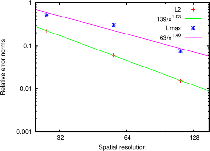
| Figure 54: Accuracy of the solution as a function of the level of refinement. |
4.1.2 PASS:
Numerical viscosity for vorticity/streamfunction formulation
-
Author
- Stéphane Popinet
- Command
- sh ../reynolds.sh stream.gfs 1
- Version
- 110610
- Required files
- stream.gfs (view) (download)
div5.ref div6.ref div7.ref reynolds.ref
- Running time
- 1 minutes 27 seconds
Same as the previous test but using a vorticity/streamfunction formulation.
| Figure 55: Evolution of the maximum divergence. |
| Figure 56: Evolution of the L2 norm of the divergence. |
| Figure 57: Evolution of the kinetic energy. |
| Figure 58: Equivalent Reynolds number as a function of resolution. |
| Figure 59: Accuracy of the solution as a function of the level of refinement. |
4.1.3 PASS:
Numerical viscosity for the skew-symmetric scheme
-
Author
- Daniel Fuster
- Command
- sh skew.sh skew.gfs 1
- Version
- 110723
- Required files
- skew.gfs (view) (download)
skew.sh div5.ref div6.ref div7.ref reynolds.ref
- Running time
- 1 minutes 17 seconds
Same as the previous test but using the skew-symmetric module.
| Figure 60: Evolution of the maximum divergence. |
| Figure 61: Evolution of the L2 norm of the divergence. |
| Figure 62: Evolution of the kinetic energy. |
| Figure 63: Accuracy of the solution as a function of the level of refinement. |
4.1.4 PASS:
Numerical viscosity for the skew-symmetric scheme with refined box
-
Author
- Daniel Fuster
- Command
- sh skew.sh skewbox.gfs 1
- Version
- 120229
- Required files
- skewbox.gfs (view) (download)
skew.sh error.ref
- Running time
- 12 minutes 28 seconds
The skew-symmetric module with AMR.
| Figure 64: Evolution of the kinetic energy. |
| Figure 65: Accuracy of the solution as a function of the level of refinement. |