Another of the test cases presented in Popinet [31], initially used by Almgren et al. [1], this convergence test illustrates the second-order accuracy of Gerris when refinement is placed appropriately, either through static refinement or dynamic adaptive refinement.
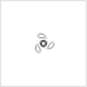
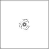
Four vortices are placed in the unit-square, centred at (0,0), (0.09,0), (−0.045,0.045√3) and (−0.045, −0.045√3) and of strengths −150, 50, 50, 50 respectively. The profile of each vortex centred around (xi,yi) is
| , |
where ri=√(x−xi)2+(y−yi)2. To initialise the velocity field, we use this vorticity as the source term in the Poisson equation for the streamfunction ψ
| ∇2ψ=||∇×U||. |
Each component of the velocity field is then calculated from the streamfunction. No-flow boundary conditions are used on the four sides of the domain and the simulations are ran to t=0.25 using a CFL of 0.9.
Two different discretisations are used, each time with up to L levels of refinement: a grid using static refinement in concentric circles of decreasing radius and a grid using dynamic adaptive refinement. The “circle” grid is constructed by starting from a uniform grid with four levels of refinement and by successively adding one level to all the cells contained within circles centred on the origin and of radii:
For the dynamically refined grid, the vorticity-based criterion is applied at every timestep with a threshold τ=4×10⁻³. As we do not have an analytical solution for this problem, Richardson extrapolation is used.
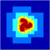
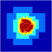
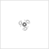
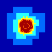
Figure 66 illustrates the evolution of the vorticity and of the adaptively refined grid for L=8. The most refined level closely follows the three outer vortices as they orbit the central one. Far from the vortices, a very coarse mesh is used (l=3). One may note a few isolated patches of refinement scattered at the periphery of the outer vortices. They are due to the numerical noise added to the vorticity by the interpolation procedure necessary to fill in velocity values for newly created cells. This could be improved by using higher-order interpolants.
Table 4 summarises the results obtained for the first twelve calculations. For fine enough grids close to second-order convergence is obtained for both norms and for the two discretisations used. The norms of the error on the various grids are also comparable for a given resolution.
Table 4: Errors and convergence orders in the x-component of the velocity for the four-way vortex merging problem. The reference solution values are given in blue.
Domain L2 L=6 O2 L=7 O2 L=8 Circle 2.63e-02 1.32 1.06e-02 1.98 2.69e-03 2.63e-02 1.32 1.06e-02 1.98 2.69e-03 Adaptive 2.56e-02 1.25 1.08e-02 1.93 2.82e-03 2.56e-02 1.25 1.08e-02 1.93 2.82e-03 Domain L∞ L=6 O∞ L=7 O∞ L=8 Circle 4.56e-01 1.28 1.88e-01 1.95 4.87e-02 4.56e-01 1.28 1.88e-01 1.95 4.87e-02 Adaptive 4.46e-01 1.19 1.96e-01 1.98 4.94e-02 4.46e-01 1.19 1.96e-01 1.98 4.94e-02
Figure 66: Contour plots of vorticity (left) and adaptive grids used (right) for the four-way vortex merging calculation.
t=0.05 t=0.15 t=0.25