The shallow-water equations are solved using the "ocean" version of Gerris. The tidal elevations for the lunar (M2) component obtained from a larger-area tidal model are imposed as conditions on the boundaries of the domain.
The comments in the tides.sh script describe how to generate the appropriate GTS files from the tidal elevation and bathymetry data.
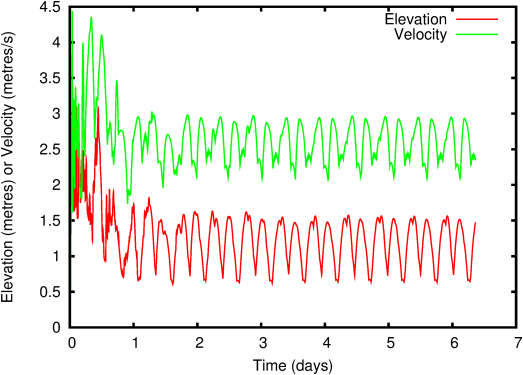
After an initial transient (t < ≈ 1 day) due to relaxation of the model toward a state consistent with the mathematical model and with the imposed boundary conditions, the model reaches a periodic regime (Figure 32).
Online harmonic decomposition can then be used to extract the amplitudes and phases of the computed M2 tidal components. The simulation stops automatically when convergence of the harmonic decomposition is reached (Figure 33).
Figure 33: Convergence of the maximum tidal amplitude (estimated from harmonic decomposition) with time. 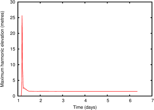
The final tidal amplitudes and phases are illustrated in Figures 34 and 35 respectively. The harmonic decomposition is also applied to the velocity field. The results can be represented as tidal ellipses (Figure 36) and residual currents (Figure 37).
Note that the results for this simulation will not be as good as these described in Rym Msadek’s technical report because iterative Flather conditions have not been applied. See the report for details.
Figure 34: Tidal amplitude estimated from the harmonic decomposition. Dark red is 1.4 metres, dark blue is 0. 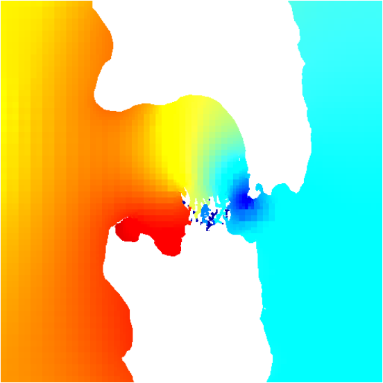
Figure 35: Tidal phase estimated from the harmonic decomposition. Dark red is 180 degrees, dark blue -180 degrees. 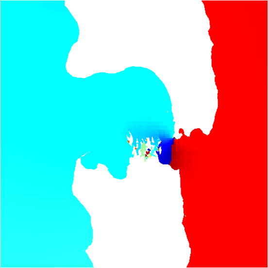
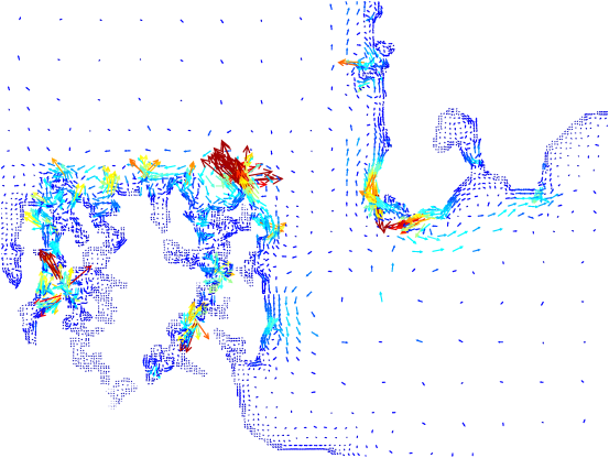
Figure 36: Detail of tidal ellipses estimated from the harmonic decomposition coloured according to maximum current speed. Dark red is 2 metres/sec, dark blue is zero. 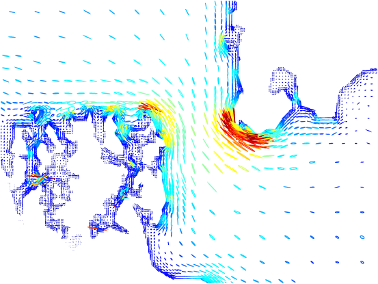
Figure 37: Detail of residual tidal currents estimated from the harmonic decomposition coloured according to residual current speed. Dark red is 0.6 metres/sec, dark blue is zero.